Next: 3.4 Discussion and Exercises Up: 3. Linked Lists Previous: 3.2 : A Doubly-Linked Contents
One of the drawbacks of linked lists (besides the time it takes to access
elements that are deep within the list) is their space usage. Each node
in a
![]() requires an additional two references to the next and
previous nodes in the list. Two of the fields in a
requires an additional two references to the next and
previous nodes in the list. Two of the fields in a
![]() are dedicated
to maintaining the list and only one of the fields is for storing data!
are dedicated
to maintaining the list and only one of the fields is for storing data!
An
![]() (space-efficient list) reduces this wasted space using
a simple idea: Rather than store individual elements in a
(space-efficient list) reduces this wasted space using
a simple idea: Rather than store individual elements in a
![]() ,
we store a block (array) containing several items. More precisely, an
,
we store a block (array) containing several items. More precisely, an
![]() is parameterized by a block size
is parameterized by a block size
![]() . Each individual
node in an
. Each individual
node in an
![]() stores a block that can hold up to
stores a block that can hold up to
![]() elements.
elements.
It will turn out, for reasons that become clear later, that it will
be helpful if we can do
![]() operations on each block. The data
structure we choose for this is a
operations on each block. The data
structure we choose for this is a
![]() (bounded deque), derived
from the
(bounded deque), derived
from the
![]() structure described in Section 2.4.
The
structure described in Section 2.4.
The
![]() differs from the
differs from the
![]() in one small way: When a
new
in one small way: When a
new
![]() is created, the size of the backing array
is created, the size of the backing array
![]() is fixed at
is fixed at
![]() and it never grows or shrinks.
The important property of a
and it never grows or shrinks.
The important property of a
![]() is that it allows for the addition or
removal of elements at either the front or back in constant time. This
will be useful as elements are shifted from one block to another.
is that it allows for the addition or
removal of elements at either the front or back in constant time. This
will be useful as elements are shifted from one block to another.
  class BDeque : public ArrayDeque<T> {
  public:
    BDeque(int b) {
      n = 0;
      j = 0;
      array<int> z(b+1);
      a = z;
    }
    ~BDeque() { }
    // C++ Question: Why is this necessary?
    void add(int i, T x) {
      ArrayDeque<T>::add(i, x);
    }
    bool add(T x) {
      ArrayDeque<T>::add(size(), x);
      return true;
    }
    void resize() {}
  };
An
![]() is then a doubly-linked list of blocks:
is then a doubly-linked list of blocks:
  class Node {
  public:
    BDeque d;
    Node *prev, *next;
    Node(int b) : d(b) { }
  };
  int n;
  Node dummy;
An
![]() places very tight restrictions on the number of elements
in a block: Unless a block is the last block, then that block contains
at least
places very tight restrictions on the number of elements
in a block: Unless a block is the last block, then that block contains
at least
![]() and at most
and at most
![]() elements. This means that, if an
elements. This means that, if an
![]() contains
contains
![]() elements, then it has at most
elements, then it has at most
The first challenge we face with an
![]() is finding the list item
with a given index
is finding the list item
with a given index
![]() . Note that the location of an element consists
of two parts: The node
. Note that the location of an element consists
of two parts: The node
![]() that contains the block that contains the
element as well as the index
that contains the block that contains the
element as well as the index
![]() of the element within its block.
of the element within its block.
  class Location {
  public:
    Node *u;
    int j;
    Location() { }
    Location(Node *u, int j) {
      this->u = u;
      this->j = j;
    }
  };
To find the block that contains a particular element, we proceed in the
same way as in a
![]() . We either start at the front of the list and
traverse in the forward direction or at the back of the list and traverse
backwards until we reach the node we want. The only difference is that,
each time we move from one node to the next, we skip over a whole block
of elements.
. We either start at the front of the list and
traverse in the forward direction or at the back of the list and traverse
backwards until we reach the node we want. The only difference is that,
each time we move from one node to the next, we skip over a whole block
of elements.
  void getLocation(int i, Location &ell) {
    if (i < n / 2) {
      Node *u = dummy.next;
      while (i >= u->d.size()) {
        i -= u->d.size();
        u = u->next;
      }
      ell.u = u;
      ell.j = i;
    } else {
      Node *u = &dummy;
      int idx = n;
      while (i < idx) {
        u = u->prev;
        idx -= u->d.size();
      }
      ell.u = u;
      ell.j = i - idx;
    }
  }
Remember that, with the exception of at most one block, each block
contains at least
![]() elements, so each step in our search gets
us
elements, so each step in our search gets
us
![]() elements closer to the element we are looking for. If we
are searching forward, this means we reach the node we want after
elements closer to the element we are looking for. If we
are searching forward, this means we reach the node we want after
![]() steps. If we search backwards, we reach the node we want
after
steps. If we search backwards, we reach the node we want
after
![]() steps. The algorithm takes the smaller of
these two quantities depending on the value of
steps. The algorithm takes the smaller of
these two quantities depending on the value of
![]() , so the time to locate
the item with index
, so the time to locate
the item with index
![]() is
is
![]() .
.
Once we know how to locate the item with index
![]() , the
, the
![]() and
and
![]() operations translate into getting or setting a particular
index in the correct block:
operations translate into getting or setting a particular
index in the correct block:
  T get(int i) {
    Location l;
    getLocation(i, l);
    return l.u->d.get(l.j);
  }
  T set(int i, T x) {
    Location l;
    getLocation(i, l);
    T y = l.u->d.get(l.j);
    l.u->d.set(l.j, x);
    return y;
  }
The running times of these operations are dominated by the time it takes
to locate the item, so they also run in
![]() time.
time.
Things start to get complicated when adding elements to an
![]() .
Before considering the general case, we consider the easier operation,
.
Before considering the general case, we consider the easier operation,
![]() , in which
, in which
![]() is added to the end of the list. If the last
block is full (or does not exist because there are no blocks yet),
then we first allocate a new block and append it to the list of blocks.
Now that we are sure that the last block exists and is not full, we
append
is added to the end of the list. If the last
block is full (or does not exist because there are no blocks yet),
then we first allocate a new block and append it to the list of blocks.
Now that we are sure that the last block exists and is not full, we
append
![]() to the last block.
to the last block.
  void add(T x) {
    Node *last = dummy.prev;
    if (last == &dummy || last->d.size() == b+1) {
      last = addBefore(&dummy);
    }
    last->d.add(x);
    n++;
  }
Things get more complicated when we add to the interior of the list
using
![]() . We first locate
. We first locate
![]() to get the node
to get the node
![]() whose block
contains the
whose block
contains the
![]() th list item. The problem is that we want to insert
th list item. The problem is that we want to insert
![]() into
into
![]() 's block, but we have to be prepared for the case where
's block, but we have to be prepared for the case where
![]() 's block already contains
's block already contains
![]() elements, so that it is full and
there is no room for
elements, so that it is full and
there is no room for
![]() .
.
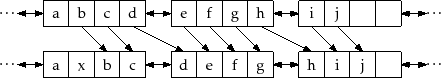
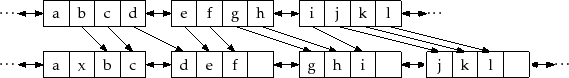
Let
![]() denote
denote
![]() ,
,
![]() ,
,
![]() ,
and so on. We explore
,
and so on. We explore
![]() looking for a node
that can provide space for
looking for a node
that can provide space for
![]() . Three cases can occur during our
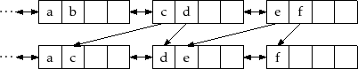
space exploration (see Figure 3.4):
. Three cases can occur during our
space exploration (see Figure 3.4):
|
  void add(int i, T x) {
    if (i == n) {
      add(x);
      return;
    }
    Location l; getLocation(i, l);
    Node *u = l.u;
    int r = 0;
    while (r < b && u != &dummy && u->d.size() == b+1) {
      u = u->next;
      r++;
    }
    if (r == b) {      // found b blocks each with b+1 elements
      spread(l.u);
      u = l.u;
    }
    if (u == &dummy) {  // ran off the end of the list - add new node
      u = addBefore(u);
    }
    while (u != l.u) { // work backwards, shifting an element at each step
      u->d.add(0, u->prev->d.remove(u->prev->d.size()-1));
      u = u->prev;
    }
    u->d.add(l.j, x);
    n++;
  }
The running time of the
![]() operation depends on which of
the three cases above occurs. Cases 1 and 2 involve examining and
shifting elements through at most
operation depends on which of
the three cases above occurs. Cases 1 and 2 involve examining and
shifting elements through at most
![]() blocks and take
blocks and take
![]() time.
Case 3 involves calling the
time.
Case 3 involves calling the
![]() method, which moves
method, which moves
![]() elements and takes
elements and takes
![]() time. If we ignore the cost of Case 3
(which we will account for later with amortization) this means that
the total running time to locate
time. If we ignore the cost of Case 3
(which we will account for later with amortization) this means that
the total running time to locate
![]() and perform the insertion of
and perform the insertion of
![]() is
is
![]() .
.
Removing an element, using the
![]() method from an
method from an
![]() is similar to adding an element. We first locate the node
is similar to adding an element. We first locate the node
![]() that
contains the element with index
that
contains the element with index
![]() . Now, we have to be prepared for
the case where we cannot remove an element from
. Now, we have to be prepared for
the case where we cannot remove an element from
![]() without causing
without causing
![]() 's
block to have size less than
's
block to have size less than
![]() , which is not allowed.
, which is not allowed.
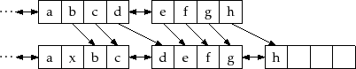
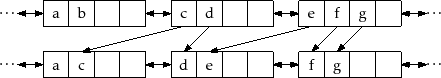
Again, let
![]() denote
denote
![]() ,
,
![]() ,
,
![]() ,
We examine
,
We examine
![]() in order looking for a node from
which we can borrow an element to make the size of
in order looking for a node from
which we can borrow an element to make the size of
![]() 's block larger
than
's block larger
than
![]() . There are three cases to consider
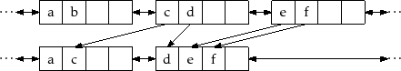
(see Figure 3.5):
. There are three cases to consider
(see Figure 3.5):
|
  T remove(int i) {
    Location l; getLocation(i, l);
    T y = l.u->d.get(l.j);
    Node *u = l.u;
    int r = 0;
    while (r < b && u != &dummy && u->d.size() == b - 1) {
      u = u->next;
      r++;
    }
    if (r == b) { // found b blocks each with b-1 elements
      gather(l.u);
    }
    u = l.u;
    u->d.remove(l.j);
    while (u->d.size() < b - 1 && u->next != &dummy) {
      u->d.add(u->next->d.remove(0));
      u = u->next;
    }
    if (u->d.size() == 0)
      remove(u);
    n--;
    return y;
  }
Like the
![]() operation, the running time of the
operation, the running time of the
![]() operation is
operation is
![]() if we ignore the cost of
the
if we ignore the cost of
the
![]() method that occurs in Case 3.
method that occurs in Case 3.
Next, we consider the cost of the
![]() and
and
![]() methods that may be executed by the
methods that may be executed by the
![]() and
and
![]() methods. For completeness, here they are:
methods. For completeness, here they are:
  void spread(Node *u) {
    Node *w = u;
    for (int j = 0; j < b; j++) {
      w = w->next;
    }
    w = addBefore(w);
    while (w != u) {
      while (w->d.size() < b)
        w->d.add(0, w->prev->d.remove(w->prev->d.size()-1));
      w = w->prev;
    }
  }
  void gather(Node *u) {
    Node *w = u;
    for (int j = 0; j < b-1; j++) {
      while (w->d.size() < b)
        w->d.add(w->next->d.remove(0));
      w = w->next;
    }
    remove(w);
  }
The running time of each of these methods is dominated by the two
nested loops. Both the inner loop and outer loop execute at most
![]() times, so the total running time of each of these methods
is
times, so the total running time of each of these methods
is
![]() . However, the following lemma shows that
these methods execute on at most one out of every
. However, the following lemma shows that
these methods execute on at most one out of every
![]() calls to
calls to
![]() or
or
![]() .
.
Notice that, if Case 1 occurs during the
![]() method, then
only one node,
method, then
only one node,
![]() has the size of its block changed. Therefore,
at most one node, namely
has the size of its block changed. Therefore,
at most one node, namely
![]() , goes from being rugged to being
fragile. If Case 2 occurs, then a new node is created, and this node
is fragile, but no other node changes sizes, so the number of fragile
nodes increases by one. Thus, in either Case 1 or Case 2 the potential
of the SEList increases by at most 1.
, goes from being rugged to being
fragile. If Case 2 occurs, then a new node is created, and this node
is fragile, but no other node changes sizes, so the number of fragile
nodes increases by one. Thus, in either Case 1 or Case 2 the potential
of the SEList increases by at most 1.
Finally, if Case 3 occurs, it is because
![]() are all fragile nodes. Then
are all fragile nodes. Then
![]() is called and these
is called and these
![]() fragile nodes are replaced with
fragile nodes are replaced with
![]() rugged nodes. Finally,
rugged nodes. Finally,
![]() is added to
is added to
![]() 's block, making
's block, making
![]() fragile. In total the
potential decreases by
fragile. In total the
potential decreases by
![]() .
.
In summary, the potential starts at 0 (there are no nodes in the list).
Each time Case 1 or Case 2 occurs, the potential increases by at
most 1. Each time Case 3 occurs, the potential decreases by
![]() .
The potential (which counts the number of fragile nodes) is never
less than 0. We conclude that, for every occurrence of Case 3, there
are at least
.
The potential (which counts the number of fragile nodes) is never
less than 0. We conclude that, for every occurrence of Case 3, there
are at least
![]() occurrences of Case 1 or Case 2. Thus, for every
call to
occurrences of Case 1 or Case 2. Thus, for every
call to
![]() there are at least
there are at least
![]() calls to
calls to
![]() . This
completes the proof.
. This
completes the proof.
![]()
The following theorem summarizes the performance of the
![]() data
structure:
data
structure:
The space (measured in words)3.1 used by an
![]() that stores
that stores
![]() elements is
elements is
![]() .
.
The
![]() is a tradeoff between an
is a tradeoff between an
![]() and a
and a
![]() where
the relative mix of these two structures depends on the block size
where
the relative mix of these two structures depends on the block size
![]() . At the extreme
. At the extreme
![]() , each
, each
![]() node stores at most 3
values, which is really not much different than a
node stores at most 3
values, which is really not much different than a
![]() . At the other
extreme,
. At the other
extreme,
![]() , all the elements are stored in a single array,
just like in an
, all the elements are stored in a single array,
just like in an
![]() . In between these two extremes lies a
tradeoff between the time it takes to add or remove a list item and
the time it takes to locate a particular list item.
. In between these two extremes lies a
tradeoff between the time it takes to add or remove a list item and
the time it takes to locate a particular list item.