Next: 6.3 Discussion and Exercises Up: 6. Binary Trees Previous: 6.1 : A Basic Contents
A
![]() is a special kind of binary tree in which each node,
is a special kind of binary tree in which each node,
![]() ,
also stores a data value,
,
also stores a data value,
![]() , from some total order. The data values in
a binary search tree obey the binary search tree property: For
a node,
, from some total order. The data values in
a binary search tree obey the binary search tree property: For
a node,
![]() , every data value stored in the subtree rooted at
, every data value stored in the subtree rooted at
![]() is less than
is less than
![]() and every data value stored in the subtree rooted at
and every data value stored in the subtree rooted at
![]() is greater than
is greater than
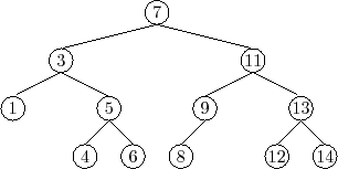
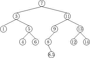
![]() . An example of a
. An example of a
![]() is shown in Figure 6.5.
is shown in Figure 6.5.
The binary search tree property is extremely useful because it allows
us to quickly locate a value,
![]() , in a binary search tree. To do this we start
searching for
, in a binary search tree. To do this we start
searching for
![]() at the root,
at the root,
![]() . When examining a node,
. When examining a node,
![]() , there
are three cases:
, there
are three cases:
  T findEQ(T x) {
    Node *w = r;
    while (w != nil) {
      int comp = compare(x, w->x);
      if (comp < 0) {
        w = w->left;
      } else if (comp > 0) {
        w = w->right;
      } else {
        return w->x;
      }
    }
    return null;
  }
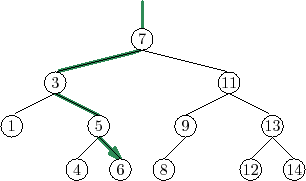
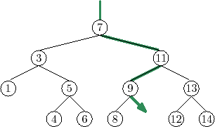
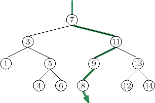
Two examples of searches in a binary search tree are shown in
Figure 6.6. As the second example shows, even if we don't find
![]() in the tree, we still gain some valuable information. If we look at
the last node,
in the tree, we still gain some valuable information. If we look at
the last node,
![]() , at which Case 1 occurred, we see that
, at which Case 1 occurred, we see that
![]() is the smallest
value in the tree that is greater than
is the smallest
value in the tree that is greater than
![]() . Similarly, the last node
at which Case 2 occurred contains the largest value in the tree that is
less than
. Similarly, the last node
at which Case 2 occurred contains the largest value in the tree that is
less than
![]() . Therefore, by keeping track of the last node,
. Therefore, by keeping track of the last node,
![]() ,
at which Case 1 occurs, a
,
at which Case 1 occurs, a
![]() can implement the
can implement the
![]() operation that returns the smallest value stored in the tree that is
greater than or equal to
operation that returns the smallest value stored in the tree that is
greater than or equal to
![]() :
:
  T find(T x) {
    Node *w = r, *z = nil;
    while (w != nil) {
      int comp = compare(x, w->x);
      if (comp < 0) {
        z = w;
        w = w->left;
      } else if (comp > 0) {
        w = w->right;
      } else {
        return w->x;
      }
    }
    return z == nil ? null : z->x;
  }
|
To add a new value,
![]() , to a
, to a
![]() , we first search for
, we first search for
![]() . If we find it, then there is no need to insert it. Otherwise,
we store
. If we find it, then there is no need to insert it. Otherwise,
we store
![]() at a leaf child of the last node,
at a leaf child of the last node,
![]() , encountered during the
search for
, encountered during the
search for
![]() . Whether the new node is the left or right child of
. Whether the new node is the left or right child of
![]() depends on the result of comparing
depends on the result of comparing
![]() and
and
![]() .
.
  bool add(T x) {
    Node *p = findLast(x);
    Node *u = new Node;
    u->x = x;
    return addChild(p, u);
  }
  Node* findLast(T x) {
    Node *w = r, *prev = nil;
    while (w != nil) {
      prev = w;
      int comp = compare(x, w->x);
      if (comp < 0) {
        w = w->left;
      } else if (comp > 0) {
        w = w->right;
      } else {
        return w;
      }
    }
    return prev;
  }
  bool addChild(Node *p, Node *u) {
      if (p == nil) {
        r = u;              // inserting into empty tree
      } else {
        int comp = compare(u->x, p->x);
        if (comp < 0) {
          p->left = u;
        } else if (comp > 0) {
          p->right = u;
        } else {
          return false;   // u.x is already in the tree
        }
        u->parent = p;
      }
      n++;
      return true;
    }
An example is shown in Figure 6.7. The most time-consuming
part of this process is the initial search for
Deleting a value stored in a node,
![]() , of a
, of a
![]() is a
little more difficult. If
is a
little more difficult. If
![]() is a leaf, then we can just detach
is a leaf, then we can just detach
![]() from its parent. Even better: If
from its parent. Even better: If
![]() has only one child, then we can
splice
has only one child, then we can
splice
![]() from the tree by having
from the tree by having
![]() adopt
adopt
![]() 's child:
's child:
  void splice(Node *u) {
    Node *s, *p;
    if (u->left != nil) {
      s = u->left;
    } else {
      s = u->right;
    }
    if (u == r) {
      r = s;
      p = nil;
    } else {
      p = u->parent;
      if (p->left == u) {
        p->left = s;
      } else {
        p->right = s;
      }
    }
    if (s != nil) {
      s->parent = p;
    }
    n--;
  }
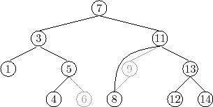
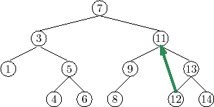
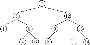
Things get tricky, though, when
![]() has two children. In this case,
the simplest thing to do is to find a node,
has two children. In this case,
the simplest thing to do is to find a node,
![]() , that has less than
two children such that we can replace
, that has less than
two children such that we can replace
![]() with
with
![]() . To maintain
the binary search tree property, the value
. To maintain
the binary search tree property, the value
![]() should be close to the
value of
should be close to the
value of
![]() . For example, picking
. For example, picking
![]() such that
such that
![]() is the smallest
value greater than
is the smallest
value greater than
![]() will do. Finding the node
will do. Finding the node
![]() is easy; it is
the smallest value in the subtree rooted at
is easy; it is
the smallest value in the subtree rooted at
![]() . This node can
be easily removed because it has no left child. (See Figure 6.9)
. This node can
be easily removed because it has no left child. (See Figure 6.9)
  void remove(Node *u) {
    if (u->left == nil || u->right == nil) {
      splice(u);
      delete u;
    } else {
      Node *w = u->right;
      while (w->left != nil)
        w = w->left;
      u->x = w->x;
      splice(w);
      delete w;
    }
  }
|
The
![]() ,
,
![]() , and
, and
![]() operations in a
operations in a
![]() each involve following a path from the root of the
tree to some node in the tree. Without knowing more about the shape of
the tree it is difficult to say much about the length of this path,
except that it is less than
each involve following a path from the root of the
tree to some node in the tree. Without knowing more about the shape of
the tree it is difficult to say much about the length of this path,
except that it is less than
![]() , the number of nodes in the tree.
The following (unimpressive) theorem summarizes the performance of the
, the number of nodes in the tree.
The following (unimpressive) theorem summarizes the performance of the
![]() data structure:
data structure:
Theorem 6.1 compares poorly with Theorem 4.1, which shows
that the
![]() structure can implement the
structure can implement the
![]() interface
with
interface
with
![]() expected time per operation. The problem with the
expected time per operation. The problem with the
![]() structure is that it can become unbalanced.
Instead of looking like the tree in Figure 6.5 it can look like a long
chain of
structure is that it can become unbalanced.
Instead of looking like the tree in Figure 6.5 it can look like a long
chain of
![]() nodes, all but the last having exactly one child.
nodes, all but the last having exactly one child.
There are a number of ways of avoiding unbalanced binary search
trees, all of which lead to data structures that have
![]() time operations. In we show how
time operations. In we show how
![]() expected time operations can be achieved with randomization.
In we show how
expected time operations can be achieved with randomization.
In we show how
![]() amortized
time operations can be achieved with partial rebuilding operations.
In we show how
amortized
time operations can be achieved with partial rebuilding operations.
In we show how
![]() worst-case
time operations can be achieved by simulating a tree that is not binary:
a tree in which nodes can have up to four children.
worst-case
time operations can be achieved by simulating a tree that is not binary:
a tree in which nodes can have up to four children.
opendatastructures.org