Next: 5.2 LinearHashTable: Linear Probing Up: 5. Hash Tables Previous: 5. Hash Tables Contents Index
A ChainedHashTable data structure uses hashing with chaining to store
data as an array,
![]() , of lists. An integer,
, of lists. An integer,
![]() , keeps track of the
total number of items in all lists (see Figure 5.1):
, keeps track of the
total number of items in all lists (see Figure 5.1):
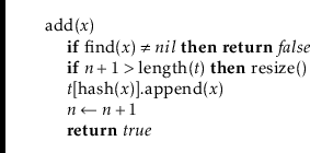
To add an element,
![]() , to the hash table, we first check if
the length of
, to the hash table, we first check if
the length of
![]() needs to be increased and, if so, we grow
needs to be increased and, if so, we grow
![]() .
With this out of the way we hash
.
With this out of the way we hash
![]() to get an integer,
to get an integer,
![]() , in the
range
, in the
range
![]() , and we append
, and we append
![]() to the list
to the list
![]() :
:
Growing the table,
if necessary, involves doubling the length of
![]() and reinserting
all elements into the new table. This strategy is exactly the same
as the one used in the implementation of ArrayStack and the same
result applies: The cost of growing is only constant when amortized
over a sequence of insertions (see Lemma 2.1 on
page
and reinserting
all elements into the new table. This strategy is exactly the same
as the one used in the implementation of ArrayStack and the same
result applies: The cost of growing is only constant when amortized
over a sequence of insertions (see Lemma 2.1 on
page ![[*]](crossref.png) ).
).
Besides growing, the only other work done when adding a new value
![]() to a
ChainedHashTable involves appending
to a
ChainedHashTable involves appending
![]() to the list
to the list
![]() . For
any of the list implementations described in Chapters 2
or 3, this takes only constant time.
. For
any of the list implementations described in Chapters 2
or 3, this takes only constant time.
To remove an element,
![]() , from the hash table, we iterate over the list
, from the hash table, we iterate over the list
![]() until we find
until we find
![]() so that we can remove it:
so that we can remove it:
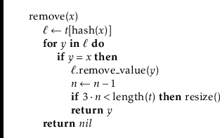
This takes
![]() time, where
time, where
![]() denotes the length
of the list stored at
denotes the length
of the list stored at
![]() .
.
Searching for the element
![]() in a hash table is similar. We perform
a linear search on the list
in a hash table is similar. We perform
a linear search on the list
![]() :
:
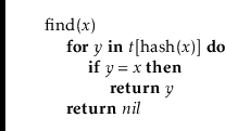
Again, this takes time proportional to the length of the list
![]() .
.
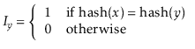
The performance of a hash table depends critically on the choice of the
hash function. A good hash function will spread the elements evenly
among the
![]() lists, so that the expected size of the list
lists, so that the expected size of the list
![]() is
is
![]() . On the other hand, a bad
hash function will hash all values (including
. On the other hand, a bad
hash function will hash all values (including
![]() ) to the same table
location, in which case the size of the list
) to the same table
location, in which case the size of the list
![]() will be
will be
![]() .
In the next section we describe a good hash function.
.
In the next section we describe a good hash function.
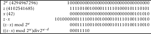
Multiplicative hashing is an efficient method of generating hash
values based on modular arithmetic (discussed in Section 2.3)
and integer division. It uses the ![]() operator, which calculates
the integral part of a quotient, while discarding the remainder.
Formally, for any integers
operator, which calculates
the integral part of a quotient, while discarding the remainder.
Formally, for any integers ![]() and
and ![]() ,
,
![]() .
.
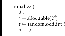
In multiplicative hashing, we use a hash table of size
![]() for some
integer
for some
integer
![]() (called the dimension). The formula for hashing an
integer
(called the dimension). The formula for hashing an
integer
![]() is
is
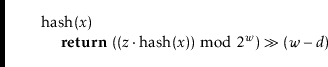
The following lemma, whose proof is deferred until later in this section, shows that multiplicative hashing does a good job of avoiding collisions:
With Lemma 5.1, the performance of
![]() , and
, and
![]() are easy to analyze:
are easy to analyze:
![$\displaystyle \mathrm{E}\left[\ensuremath{\ensuremath{\ensuremath{\mathit{n}}}}...
...mathit{y}}}}\in S} I_{\ensuremath{\ensuremath{\ensuremath{\mathit{y}}}}}\right]$](img1990.png) |
|||
![$\displaystyle \ensuremath{\ensuremath{\ensuremath{\mathit{n}}}}_{\ensuremath{\e...
...{y}}}}\in S} \mathrm{E}[I_{\ensuremath{\ensuremath{\ensuremath{\mathit{y}}}}} ]$](img1992.png) |
|||
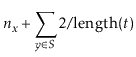 |
|||
 |
|||
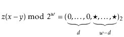
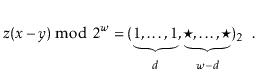
Now, we want to prove Lemma 5.1, but first we need a
result from number theory. In the following proof, we use the notation
![]() to denote
to denote
![]() , where each
, where each ![]() is a bit, either 0 or 1. In other words,
is a bit, either 0 or 1. In other words,
![]() is
the integer whose binary representation is given by
is
the integer whose binary representation is given by
![]() .
We use
.
We use ![]() to denote a bit of unknown value.
to denote a bit of unknown value.
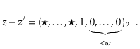
Suppose, for the sake of contradiction, that there are two such values
![]() and
and
![]() , with
, with
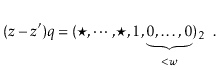
![]() . Then
. Then
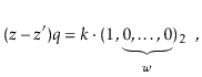
Furthermore ![]() , since
, since ![]() and
and
![]() . Since
. Since ![]() is odd, it has no trailing 0's in its binary representation:
is odd, it has no trailing 0's in its binary representation:
The utility of Lemma 5.3 comes from the following
observation: If
![]() is chosen uniformly at random from
is chosen uniformly at random from ![]() , then
, then
![]() is uniformly distributed over
is uniformly distributed over ![]() . In the following proof, it helps
to think of the binary representation of
. In the following proof, it helps
to think of the binary representation of
![]() , which consists of
, which consists of
![]() random bits followed by a 1.
random bits followed by a 1.
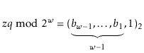
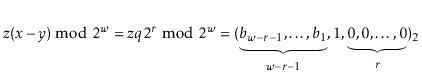
Let ![]() be the unique odd integer such that
be the unique odd integer such that
![]() for some integer
for some integer ![]() . By
Lemma 5.3, the binary representation of
. By
Lemma 5.3, the binary representation of
![]() has
has
![]() random bits, followed by a 1:
random bits, followed by a 1:
The following theorem summarizes the performance of a ChainedHashTable data structure:
Furthermore, beginning with an empty ChainedHashTable, any sequence of
![]()
![]() and
and
![]() operations results in a total of
operations results in a total of ![]() time spent during all calls to
time spent during all calls to
![]() .
.
![\includegraphics[width=\textwidth ]{figs-python/chainedhashtable}](img1904.png)