Next: 1.2 Mathematical Background Up: 1. Introduction Previous: 1. Introduction Contents
In discussing data structures, it is important to understand the difference between a data structure's interface and its implementation. An interface describes what a data structure does, while an implementation describes how the data structure does it.
An interface, sometimes also called an abstract data type, defines the set of operations supported by a data structure and the semantics, or meaning, of those operations. An interface tells us nothing about how the data structure implements these operations, it only provides the list of supported operations along with specifications about what types of arguments each operation accepts and the value returned by each operation.
A data structure implementation on the other hand, includes the
internal representation of the data structure as well as the definitions
of the algorithms that implement the operations supported by the data
structure. Thus, there can be many implementations of a single interface.
For example, in Chapter 2, we will see implementations of the
![]() interface using arrays and in Chapter 3 we will
see implementations of the
interface using arrays and in Chapter 3 we will
see implementations of the
![]() interface using pointer-based data
structures. Each implements the same interface,
interface using pointer-based data
structures. Each implements the same interface,
![]() ,
but in different ways.
,
but in different ways.
The
![]() interface represents a collection of elements to which we
can add elements and remove the next element. More precisely, the operations
supported by the
interface represents a collection of elements to which we
can add elements and remove the next element. More precisely, the operations
supported by the
![]() interface are
interface are
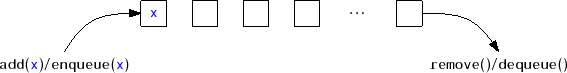
A FIFO (first-in-first-out)
![]() , illustrated in Figure 1.1,
removes items in the same order they were added, much in the same
way a queue (or line-up) works when checking out at a cash register
in a grocery store. This is the most common kind of
, illustrated in Figure 1.1,
removes items in the same order they were added, much in the same
way a queue (or line-up) works when checking out at a cash register
in a grocery store. This is the most common kind of
![]() so the
qualifier FIFO is often ommitted. In other texts, the
so the
qualifier FIFO is often ommitted. In other texts, the
![]() and
and
![]() operations on a FIFO
operations on a FIFO
![]() are often called
are often called
![]() and
and
![]() , respectively.
, respectively.
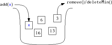
A priority
![]() , illustrated in Figure 1.2, always
removes the smallest element from the
, illustrated in Figure 1.2, always
removes the smallest element from the
![]() , breaking ties arbitrarily.
This is similar to the way patients are triaged in a hospital emergency
room. As patients arrive they are evaluated and then placed in a waiting
room. When a doctor becomes available they first treat the patient with
the most life-threatening condition. The
, breaking ties arbitrarily.
This is similar to the way patients are triaged in a hospital emergency
room. As patients arrive they are evaluated and then placed in a waiting
room. When a doctor becomes available they first treat the patient with
the most life-threatening condition. The
![]() operation on a
priority
operation on a
priority
![]() is usually called
is usually called
![]() in other texts.
in other texts.
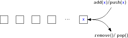
A very common queueing discipline is the LIFO (last-in-first-out)
discipline, illustrated in Figure 1.3. In a LIFO Queue,
the most recently added element is the next one removed. This is best
visualized in terms of a stack of plates; plates are placed on the top of
the stack and also removed from the top of the stack. This structure is
so common that it gets its own name:
![]() . Often, when discussing a
. Often, when discussing a
![]() , the names of
, the names of
![]() and
and
![]() are changed to
are changed to
![]() and
and
![]() ; this is to avoid confusing the LIFO and FIFO queueing
disciplines.
; this is to avoid confusing the LIFO and FIFO queueing
disciplines.
A
![]() is a generalization of both the FIFO
is a generalization of both the FIFO
![]() and LIFO
and LIFO
![]() (
(
![]() ). A
). A
![]() represents a sequence of elements, with a front
and a back. Elements can be added at the front of the sequence or
the back of the sequence. The names of the operations on a
represents a sequence of elements, with a front
and a back. Elements can be added at the front of the sequence or
the back of the sequence. The names of the operations on a
![]() are self-explanatory:
are self-explanatory:
![]() ,
,
![]() ,
,
![]() ,
and
,
and
![]() . Notice that a
. Notice that a
![]() can be implemented using only
can be implemented using only
![]() and
and
![]() while a FIFO
while a FIFO
![]() can be implemented
using only
can be implemented
using only
![]() and
and
![]() .
.
This book will talk very little about the FIFO
![]() ,
,
![]() , or
, or
![]() interfaces. This is because these interfaces are subsumed by the
interfaces. This is because these interfaces are subsumed by the
![]() interface. A
interface. A
![]() , illustrated in Figure 1.4, represents a
sequence,
, illustrated in Figure 1.4, represents a
sequence,
![]() , of values. The
, of values. The
![]() interface
includes the following operations:
interface
includes the following operations:
Although we will normally not discuss the
![]() ,
,
![]() and FIFO
and FIFO
![]() interfaces in subsequent chapters, the terms
interfaces in subsequent chapters, the terms
![]() and
and
![]() are sometimes used in the names of data structures that implement the
are sometimes used in the names of data structures that implement the
![]() interface. When this happens, it is to highlight the fact that
these data structures can be used to implement the
interface. When this happens, it is to highlight the fact that
these data structures can be used to implement the
![]() or
or
![]() interface very efficiently. For example, the
interface very efficiently. For example, the
![]() class is an
implementation of the
class is an
implementation of the
![]() interface that implements all the
interface that implements all the
![]() operations in constant time per operation.
operations in constant time per operation.
The
![]() interface represents an unordered set of unique elements,
mimicking a mathematical set. A
interface represents an unordered set of unique elements,
mimicking a mathematical set. A
![]() contains
contains
![]() distinct
elements; no element appears more than once; the elements are in no
specific order. A
distinct
elements; no element appears more than once; the elements are in no
specific order. A
![]() supports the following operations:
supports the following operations:
These definitions are a bit fussy about distinguishing
![]() , the element
we are removing or finding, from
, the element
we are removing or finding, from
![]() , the element we remove or find.
This is because
, the element we remove or find.
This is because
![]() and
and
![]() might actually be distinct objects that
are nevertheless treated as equal.
This is a very useful distinction since it allows for the creation of
dictionaries or maps that map keys onto values. This is
done by creating a compound object called a
might actually be distinct objects that
are nevertheless treated as equal.
This is a very useful distinction since it allows for the creation of
dictionaries or maps that map keys onto values. This is
done by creating a compound object called a
![]() that contains a
key and a value. Two
that contains a
key and a value. Two
![]() s are treated as equal if their
keys are equal. By storing
s are treated as equal if their
keys are equal. By storing
![]() s in a
s in a
![]() , we can find the value
associated with any key
, we can find the value
associated with any key
![]() by creating a
by creating a
![]() ,
,
![]() , with key
, with key
![]() and using the
and using the
![]() method.
method.
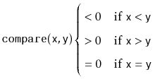
The
![]() interface represents a sorted set of elements. An
interface represents a sorted set of elements. An
![]() stores elements from some total order, so that any two elements
stores elements from some total order, so that any two elements
![]() and
and
![]() can be compared. In code examples, this will be done with a
method called
can be compared. In code examples, this will be done with a
method called
![]() in which
in which
This version of the
![]() operation is sometimes referred to
as a successor search. It differs in a fundamental way from
operation is sometimes referred to
as a successor search. It differs in a fundamental way from
![]() since it returns a meaningful result even when there is
no element in the set that is equal to
since it returns a meaningful result even when there is
no element in the set that is equal to
![]() .
.
The distinction between the
![]() and
and
![]()
![]() operations is very
important and is very often missed. The extra functionality provided
by an
operations is very
important and is very often missed. The extra functionality provided
by an
![]() usually comes with a price that includes both a larger
running time and a higher implementation complexity. For example, most
of the
usually comes with a price that includes both a larger
running time and a higher implementation complexity. For example, most
of the
![]() implementations discussed in this book all have
implementations discussed in this book all have
![]() operations with running times that are logarithmic in the size of the set.
On the other hand, the implementation of a
operations with running times that are logarithmic in the size of the set.
On the other hand, the implementation of a
![]() as a
as a
![]() in Chapter 5 has a
in Chapter 5 has a
![]() operation that runs in constant
expected time. When choosing which of these structures to use, one should
always use a
operation that runs in constant
expected time. When choosing which of these structures to use, one should
always use a
![]() unless the extra functionality offered by an
unless the extra functionality offered by an
![]() is really needed.
is really needed.
opendatastructures.org