12.3 Graph Traversal

In this section we present two algorithms for exploring a graph, starting at one of its vertices, $\mathtt{i}$, and finding all vertices that are reachable from $\mathtt{i}$. Both of these algorithms are best suited to graphs represented using an adjacency list representation. Therefore, when analyzing these algorithms we will assume that the underlying representation is as an $\mathtt{AdjacencyLists}$.

12.3.1 Breadth-First Search

The bread-first-search algorithm starts at a vertex $\mathtt{i}$ and visits, first the neighbours of $\mathtt{i}$, then the neighbours of the neighbours of $\mathtt{i}$, then the neighbours of the neighbours of the neighbours of $\mathtt{i}$, and so on.

This algorithm is a generalization of the breadth-first-search algorithm for binary trees (Section 6.1.2), and is very similar; it uses a queue, $\mathtt{q}$, that initially contains only $\mathtt{i}$. It then repeatedly extracts an element from $\mathtt{q}$ and adds its neighbours to $\mathtt{q}$, provided that these neighbours have never been in $\mathtt{q}$ before. The only major difference between breadth-first-search for graphs and for trees is that the algorithm for graphs has to ensure that it does not add the same vertex to $\mathtt{q}$ more than once. It does this by using an auxiliary boolean array, $\mathtt{seen}$, that keeps track of which vertices have already been discovered.

void bfs(Graph &g, int r) {
  bool *seen = new bool[g.nVertices()];
  SLList<int> q;
  q.add(r);
  seen[r] = true;
  while (q.size() > 0) {
    int i = q.remove();
    ArrayStack<int> edges;
    g.outEdges(i, edges);
    for (int k = 0; k < edges.size(); k++) {
      int j = edges.get(k);
      if (!seen[j]) {
        q.add(j);
        seen[j] = true;
      }
    }
  }
  delete[] seen;
}

An example of running $\mathtt{bfs(g,0)}$ on the graph from Figure 12.1 is shown in Figure 12.4. Different executions are possible, depending on the ordering of the adjacency lists; Figure 12.4 uses the adjacency lists in Figure 12.3.

Figure 12.4: An example of bread-first-search starting at node 0. Nodes are labelled with the order in which they are added to $\mathtt{q}$. Edges that result in nodes being added to $\mathtt{q}$ are drawn in black, other edges are drawn in grey.

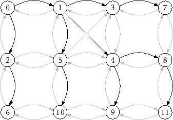
Analyzing the running-time of the $\mathtt{bfs(g,i)}$ routine is fairly straightforward. The use of the $\mathtt{seen}$ array ensures that no vertex is added to $\mathtt{q}$ more than once. Adding (and later removing) each vertex from $\mathtt{q}$ takes constant time per vertex for a total of $O(\ensuremath{\mathtt{n}})$ time. Since each vertex is processed at most once by the inner loop, each adjacency list is processed at most once, so each edge of $G$ is processed at most once. This processing, which is done in the inner loop takes constant time per iteration, for a total of $O(\ensuremath{\mathtt{m}})$ time. Therefore, the entire algorithm runs in $O(\ensuremath{\mathtt{n}} + \ensuremath{\mathtt{m}})$ time.

The following theorem summarizes the performance of the $\mathtt{bfs(g,r)}$ algorithm.

Theorem 12..3   When given as input a $\mathtt{Graph}$, $\mathtt{g}$, that is implemented using the $\mathtt{AdjacencyLists}$ data structure, the $\mathtt{bfs(g,r)}$ algorithm runs in $O(\ensuremath{\mathtt{n}} + \ensuremath{\mathtt{m}})$ time.

A breadth-first traversal has some very special properties. Calling $\mathtt{bfs(g,r)}$ will eventually enqueue (and eventually dequeue) every vertex $\mathtt{j}$ such that there is a directed path from $\mathtt{r}$ to $\mathtt{j}$. Moreover, the vertices at distance 0 from $\mathtt{r}$ ( $\mathtt{r}$ itself) will enter $\mathtt{q}$ before the vertices at distance 1, which will enter $\mathtt{q}$ before the vertices at distance 2, and so on. Thus, the $\mathtt{bfs(g,r)}$ method visits vertices in increasing order of distance from $\mathtt{r}$ and vertices that can not be reached from $\mathtt{r}$ are never output at all.

A particularly useful application of the breadth-first-search algorithm is, therefore, in computing shortest paths. To compute the shortest path from $\mathtt{r}$ to every other vertex, we use a variant of $\mathtt{bfs(g,r)}$ that uses an auxilliary array, $\mathtt{p}$, of length $\mathtt{n}$. When a new vertex $\mathtt{j}$ is added to $\mathtt{q}$, we set $\mathtt{p[j]=i}$. In this way, $\mathtt{p[j]}$ becomes the second last node on a shortest path from $\mathtt{r}$ to $\mathtt{j}$. Repeating this, by taking $\mathtt{p[p[j]}$, $\mathtt{p[p[p[j]]]}$, and so on we can reconstruct the (reversal of) a shortest path from $\mathtt{r}$ to $\mathtt{j}$.

12.3.2 Depth-First Search

The depth-first-search algorithm is similar to the standard algorithm for traversing binary trees; it first fully explores one subtree before returning to the current node and then exploring the other subtree. Another way to think of depth-first-search is by saying that it is similar to breadth-first search except that it uses a stack instead of a queue.

During the execution of the depth-first-search algorithm, each vertex, $\mathtt{i}$, is assigned a color, $\mathtt{c[i]}$: $\mathtt{white}$ if we have never seen the vertex before, $\mathtt{grey}$ if we are currently visiting that vertex, and $\mathtt{black}$ if we are done visiting that vertex. The easiest way to think of depth-first-search is as a recursive algorithm. It starts by visiting $\mathtt{r}$. When visiting a vertex $\mathtt{i}$, we first mark $\mathtt{i}$ as $\mathtt{grey}$. Next, we scan $\mathtt{i}$'s adjacency list and recursively visit any white vertex we find in this list. Finally, we are done processing $\mathtt{i}$, so we color $\mathtt{i}$ black and return.

void dfs(Graph &g, int i, char *c) {
  c[i] = grey;  // currently visiting i
  ArrayStack<int> edges;
  g.outEdges(i, edges);
  for (int k = 0; k < edges.size(); k++) {
    int j = edges.get(k);
    if (c[j] == white) {
      c[j] = grey;
      dfs(g, j, c);
    }
  }
  c[i] = black; // done visiting i
}
void dfs(Graph &g, int r) {
  char *c = new char[g.nVertices()];
  dfs(g, r, c);
  delete[] c;
}

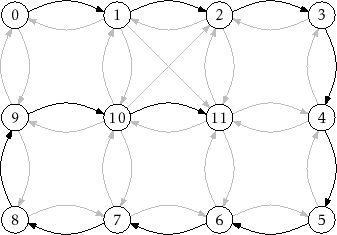
An example of the execution of this algorithm is shown in Figure 12.5

Figure 12.5: An example of depth-first-search starting at node 0. Nodes are labelled with the order in which they are processed. Edges that result in a recursive call are drawn in black, other edges are drawn in $\mathtt{grey}$.

Although depth-first-search may best be thought of as a recursive algorithm, recursion is not the best way to implement it. Indeed, the code given above will fail for many large graphs by causing a stack overflow. An alternative implementation is to replace the recursion stack with an explicit stack, $\mathtt{s}$. The following implementation does just that:

void dfs2(Graph &g, int r) {
  char *c = new char[g.nVertices()];
  SLList<int> s;
  s.push(r);
  while (s.size() > 0) {
    int i = s.pop();
    if (c[i] == white) {
      c[i] = grey;
      ArrayStack<int> edges;
      g.outEdges(i, edges);
      for (int k = 0; k < edges.size(); k++)
        s.push(edges.get(k));
    }
  }
  delete[] c;
}

In the above code, when next vertex, $\mathtt{i}$, is processed, $\mathtt{i}$ is colored $\mathtt{grey}$ and then replaced, on the stack, with its adjacent vertices. During the next iteration, one of these vertices will be visited.

Not surprisingly, the running times of $\mathtt{dfs(g,r)}$ and $\mathtt{dfs2(g,r)}$ are the same as that of $\mathtt{bfs(g,r)}$:

Theorem 12..4   When given as input a $\mathtt{Graph}$, $\mathtt{g}$, that is implemented using the $\mathtt{AdjacencyLists}$ data structure, the $\mathtt{dfs(g,r)}$ and $\mathtt{dfs2(g,r)}$ algorithms each run in $O(\ensuremath{\mathtt{n}} + \ensuremath{\mathtt{m}})$ time.

As with the breadth-first-search algorithm, there is an underlying tree associated with each execution of depth-first-search. When a node $\ensuremath{\mathtt{i}}\neq \ensuremath{\mathtt{r}}$ goes from $\mathtt{white}$ to $\mathtt{grey}$, this is because $\mathtt{dfs(g,i,c)}$ was called recursively while processing some node $\mathtt{i'}$. (In the case of $\mathtt{dfs2(g,r)}$ algorithm, $\mathtt{i}$ is one of the nodes that replaced $\mathtt{i'}$ on the stack.) If we think of $\mathtt{i'}$ as the parent of $\mathtt{i}$, then we obtain a tree rooted at $\mathtt{r}$. In Figure 12.5, this tree is a path from vertex 0 to vertex 11.

An important property of the depth-first-search algorithm is the following: Suppose that when node $\mathtt{i}$ is colored $\mathtt{grey}$, there exists a path from $\mathtt{i}$ to some other node $\mathtt{j}$ that uses only white vertices. Then $\mathtt{j}$ will be colored (first $\mathtt{grey}$ then) $\mathtt{black}$ before $\mathtt{i}$ is colored $\mathtt{black}$. (This can be proven by contradiction, by considering any path $P$ from $\mathtt{i}$ to $\mathtt{j}$.)

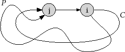
One application of this property is the detection of cycles. Refer to Figure 12.6. Consider some cycle, $C$, that can be reached from $\mathtt{r}$. Let $\mathtt{i}$ be the first node of $C$ that is colored $\mathtt{grey}$, and let $\mathtt{j}$ be the node that precedes $\mathtt{i}$ on the cycle $C$. Then, by the above property, $\mathtt{j}$ will be colored $\mathtt{grey}$ and the edge $\mathtt{(j,i)}$ will be considered by the algorithm while $\mathtt{i}$ is still $\mathtt{grey}$. Thus, the algorithm can conclude that there is a path, $P$, from $\mathtt{i}$ to $\mathtt{j}$ in the depth-first-search tree and the edge $\mathtt{(j,i)}$ exists. Therefore, $P$ is also a cycle.

Figure 12.6: The depth-first-search algorithm can be used to detect cycles in $G$.The node $\mathtt{j}$ is colored $\mathtt{grey}$ while $\mathtt{i}$ is still $\mathtt{grey}$. This implies there is a path, $P$, from $\mathtt{i}$ to $\mathtt{j}$ in the depth-first-search tree, and the edge $\mathtt{(j,i)}$ implies that $P$ is also a cycle.