Next: 7.3 Discussion and Exercises Up: 7. Random Binary Search Previous: 7.1 Random Binary Search Contents
The problem with random binary search trees is, of course, that they are
not dynamic. They don't support the
![]() or
or
![]() operations
needed to implement the SSet interface. In this section we describe
a data structure called a Treap that uses Lemma 7.1 to implement
the SSet interface.
operations
needed to implement the SSet interface. In this section we describe
a data structure called a Treap that uses Lemma 7.1 to implement
the SSet interface.
A node in a Treap is like a node in a BinarySearchTree in that it has
a data value,
![]() , but it also contains a unique numerical priority,
, but it also contains a unique numerical priority,
![]() , that is assigned at random:
, that is assigned at random:
    class Node<T> extends BinarySearchTree.BSTNode<Node<T>,T> {
        int p;
    }
In addition to being a binary search tree, the nodes in a Treap
also obey the heap property: At every node
The heap and binary search tree conditions together ensure that, once
the key (
![]() ) and priority (
) and priority (
![]() ) for each node are defined, the
shape of the Treap is completely determined. The heap property tells us that
the node with minimum priority has to be the root,
) for each node are defined, the
shape of the Treap is completely determined. The heap property tells us that
the node with minimum priority has to be the root,
![]() , of the Treap.
The binary search tree property tells us that all nodes with keys smaller
than
, of the Treap.
The binary search tree property tells us that all nodes with keys smaller
than
![]() are stored in the subtree rooted at
are stored in the subtree rooted at
![]() and all nodes
with keys larger than
and all nodes
with keys larger than
![]() are stored in the subtree rooted at
are stored in the subtree rooted at
![]() .
.
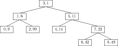
The important point about the priority values in a Treap is that they
are unique and assigned at random. Because of this, there are
two equivalent ways we can think about a Treap. As defined above, a
Treap obeys the heap and binary search tree properties. Alternatively,
we can think of a Treap as a BinarySearchTree whose nodes
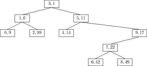
were added in increasing order of priority. For example, the Treap
in Figure 7.5 can be obtained by adding the sequence of
![]() values
values
Since the priorities are chosen randomly, this is equivalent to taking a random permutation of the keys -- in this case the permutation is
Lemma 7.2 tells us that Treaps can implement the
![]() operation efficiently. However, the real benefit of a Treap is that
it can support the
operation efficiently. However, the real benefit of a Treap is that
it can support the
![]() and
and
![]() operations. To
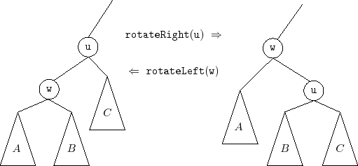
do this, it needs to perform rotations in order to maintain the heap property. Refer to Figure 7.6.
A rotation in a binary
search tree is a local modification that takes a parent
operations. To
do this, it needs to perform rotations in order to maintain the heap property. Refer to Figure 7.6.
A rotation in a binary
search tree is a local modification that takes a parent
![]() of a node
of a node
![]() and makes
and makes
![]() the parent of
the parent of
![]() , while preserving the binary search tree
property. Rotations come in two flavours: left or right
depending on whether
, while preserving the binary search tree
property. Rotations come in two flavours: left or right
depending on whether
![]() is a right or left child of
is a right or left child of
![]() , respectively.
, respectively.
The code that implements this has to handle these two possibilities
and be careful of a boundary
case (when
![]() is the root) so the actual code is a little longer than
Figure 7.6 would lead a reader to believe:
is the root) so the actual code is a little longer than
Figure 7.6 would lead a reader to believe:
    void rotateLeft(Node u) {
        Node w = u.right;
        w.parent = u.parent;
        if (w.parent != nil) {
            if (w.parent.left == u) {
                w.parent.left = w;
            } else {
                w.parent.right = w;
            }
        }
        u.right = w.left;
        if (u.right != nil) {
            u.right.parent = u;
        }
        u.parent = w;
        w.left = u;
        if (u == r) { r = w; r.parent = nil; }
    }
    void rotateRight(Node u) {
        Node w = u.left;
        w.parent = u.parent;
        if (w.parent != nil) {
            if (w.parent.left == u) {
                w.parent.left = w;
            } else {
                w.parent.right = w;
            }
        }
        u.left = w.right;
        if (u.left != nil) {
            u.left.parent = u;
        }
        u.parent = w;
        w.right = u;
        if (u == r) { r = w; r.parent = nil; }
    }
In terms of the Treap data structure, the most important property of a
rotation is that the depth of
Using rotations, we can implement the
![]() operation as follows:
We create a new node,
operation as follows:
We create a new node,
![]() , and assign
, and assign
![]() and pick a random value
for
and pick a random value
for
![]() . Next we add
. Next we add
![]() using the usual
using the usual
![]() algorithm
for a BinarySearchTree, so that
algorithm
for a BinarySearchTree, so that
![]() is now a leaf of the Treap.
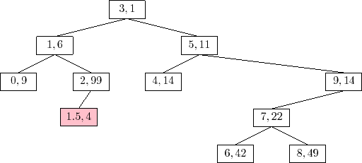
At this point, our Treap satisfies the binary search tree property,
but not necessarily the heap property. In particular, it may be the
case that
is now a leaf of the Treap.
At this point, our Treap satisfies the binary search tree property,
but not necessarily the heap property. In particular, it may be the
case that
![]() . If this is the case, then we perform a
rotation at node
. If this is the case, then we perform a
rotation at node
![]() =
=
![]() so that
so that
![]() becomes the parent of
becomes the parent of
![]() .
If
.
If
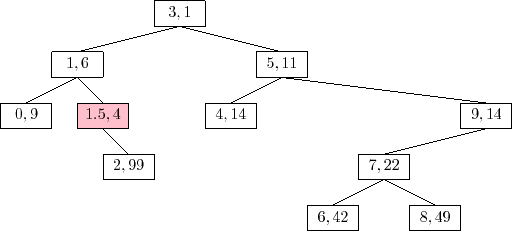
![]() continues to violate the heap property, we will have to repeat this, decreasing
continues to violate the heap property, we will have to repeat this, decreasing
![]() 's depth by one every time, until
's depth by one every time, until
![]() either becomes the root or
either becomes the root or
![]() .
.
    boolean add(T x) {
        Node<T> u = newNode();
        u.x = x;
        u.p = rand.nextInt();
        if (super.add(u)) {
            bubbleUp(u);
            return true;
        }
        return false;
    }
    void bubbleUp(Node<T> u) {
        while (u.parent != nil && u.parent.p > u.p) {
            if (u.parent.right == u) {
                rotateLeft(u.parent);
            } else {
                rotateRight(u.parent);
            }
        }
        if (u.parent == nil) {
            r = u;
        }
    }
An example of an
The running time of the
![]() operation is given by the time it
takes to follow the search path for
operation is given by the time it
takes to follow the search path for
![]() plus the number of rotations
performed to move the newly-added node,
plus the number of rotations
performed to move the newly-added node,
![]() , up to its correct location
in the Treap. By Lemma 7.2, the expected length of the
search path is at most
, up to its correct location
in the Treap. By Lemma 7.2, the expected length of the
search path is at most
![]() . Furthermore, each rotation
decreases the depth of
. Furthermore, each rotation
decreases the depth of
![]() . This stops if
. This stops if
![]() becomes the root, so
the expected number of rotations cannot exceed the expected length of
the search path. Therefore, the expected running time of the
becomes the root, so
the expected number of rotations cannot exceed the expected length of
the search path. Therefore, the expected running time of the
![]() operation in a Treap is
operation in a Treap is
![]() . (Exercise 7.3
asks you to show that the expected number of rotations performed during
an insertion is actually only
. (Exercise 7.3
asks you to show that the expected number of rotations performed during
an insertion is actually only ![]() .)
.)
The
![]() operation in a Treap is the opposite of the
operation in a Treap is the opposite of the
![]() operation. We search for the node,
operation. We search for the node,
![]() , containing
, containing
![]() and then perform
rotations to move
and then perform
rotations to move
![]() downwards until it becomes a leaf and then we
splice
downwards until it becomes a leaf and then we
splice
![]() from the Treap. Notice that, to move
from the Treap. Notice that, to move
![]() downwards, we can
perform either a left or right rotation at
downwards, we can
perform either a left or right rotation at
![]() , which will replace
, which will replace
![]() with
with
![]() or
or
![]() , respectively.
The choice is made by the first of the following that apply:
, respectively.
The choice is made by the first of the following that apply:
    boolean remove(T x) {
        Node<T> u = findLast(x);
        if (u != nil && compare(u.x, x) == 0) {
            trickleDown(u);
            splice(u);
            return true;
        }
        return false;
    }
    void trickleDown(Node<T> u) {
        while (u.left != nil || u.right != nil) {
            if (u.left == nil) {
                rotateLeft(u);
            } else if (u.right == nil) {
                rotateRight(u);
            } else if (u.left.p < u.right.p) {
                rotateRight(u);
            } else {
                rotateLeft(u);
            }
            if (r == u) {
                r = u.parent;
            }
        }
    }
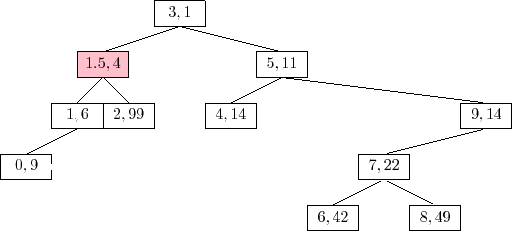
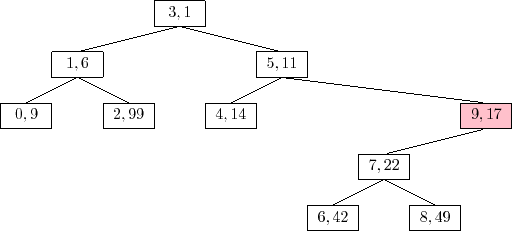
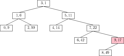
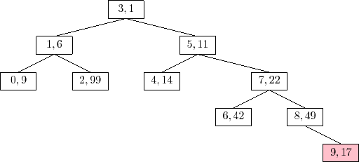
An example of the
The trick to analyze the running time of the
![]() operation is
to notice that this operation is the reverse of the
operation is
to notice that this operation is the reverse of the
![]() operation.
In particular, if we were to reinsert
operation.
In particular, if we were to reinsert
![]() , using the same priority
, using the same priority
![]() ,
then the
,
then the
![]() operation would do exactly the same number of rotations
and would restore the Treap to exactly the same state it was in before
the
operation would do exactly the same number of rotations
and would restore the Treap to exactly the same state it was in before
the
![]() operation took place. (Reading from bottom-to-top,
Figure 7.8 illustrates the insertion of the value 9 into a
Treap.) This means that the expected running time of the
operation took place. (Reading from bottom-to-top,
Figure 7.8 illustrates the insertion of the value 9 into a
Treap.) This means that the expected running time of the
![]() on a Treap of size
on a Treap of size
![]() is proportional to the expected running time
of the
is proportional to the expected running time
of the
![]() operation on a Treap of size
operation on a Treap of size
![]() . We conclude
that the expected running time of
. We conclude
that the expected running time of
![]() is
is
![]() .
.
The following theorem summarizes the performance of the Treap data structure:
It is worth comparing the Treap data structure to the SkiplistSSet
data structure. Both implement the SSet operations in
![]() expected time per operation. In both data structures,
expected time per operation. In both data structures,
![]() and
and
![]() involve a search and then a constant number of pointer changes
(see Exercise 7.3 below). Thus, for both these
structures, the expected length of the search path is the critical value
in assessing their performance. In a SkiplistSSet, the expected length
of a search path is
involve a search and then a constant number of pointer changes
(see Exercise 7.3 below). Thus, for both these
structures, the expected length of the search path is the critical value
in assessing their performance. In a SkiplistSSet, the expected length
of a search path is