Next: 4.4 Analysis of Skiplists Up: 4. Skiplists Previous: 4.2 SkiplistSSet: An Efficient Contents Index
A SkiplistList implements the List interface using a skiplist
structure. In a SkiplistList, ![]() contains the elements of the
list in the order in which they appear in the list. As in a
SkiplistSSet, elements can be added, removed, and accessed in
contains the elements of the
list in the order in which they appear in the list. As in a
SkiplistSSet, elements can be added, removed, and accessed in
![]() time.
time.
For this to be possible, we need a way to follow the search path for
the
![]() th element in
th element in ![]() . The easiest way to do this is to define
the notion of the length of an edge in some list,
. The easiest way to do this is to define
the notion of the length of an edge in some list,
![]() .
We define the length of every edge in
.
We define the length of every edge in ![]() as 1. The length of an edge,
as 1. The length of an edge,
![]() ,
in
,
in
![]() ,
,
![]() , is defined as the sum of the lengths of the edges below
, is defined as the sum of the lengths of the edges below
![]() in
in
![]() . Equivalently, the length of
. Equivalently, the length of
![]() is
the number of edges in
is
the number of edges in ![]() below
below
![]() . See Figure 4.5 for
an example of a skiplist with the lengths of its edges shown. Since the
edges of skiplists are stored in arrays, the lengths can be stored the same
way:
. See Figure 4.5 for
an example of a skiplist with the lengths of its edges shown. Since the
edges of skiplists are stored in arrays, the lengths can be stored the same
way:
The useful property of this definition of length is that, if we are
currently at a node that is at position
![]() in
in ![]() and we follow an
edge of length
and we follow an
edge of length ![]() , then we move to a node whose position, in
, then we move to a node whose position, in ![]() ,
is
,
is
![]() . In this way, while following a search path, we can keep
track of the position,
. In this way, while following a search path, we can keep
track of the position,
![]() , of the current node in
, of the current node in ![]() . When at a
node,
. When at a
node,
![]() , in
, in
![]() , we go right if
, we go right if
![]() plus the length of the edge
plus the length of the edge
![]() is less than
is less than
![]() . Otherwise, we go down into
. Otherwise, we go down into
![]() .
.
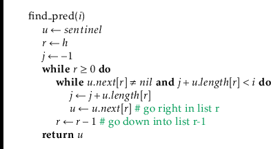
Since the hardest part of the operations
![]() and
and
![]() is
finding the
is
finding the
![]() th node in
th node in ![]() , these operations run in
, these operations run in
![]() time.
time.
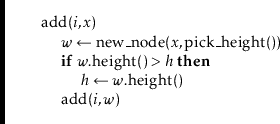
Adding an element to a SkiplistList at a position,
![]() , is fairly
simple. Unlike in a SkiplistSSet, we are sure that a new
node will actually be added, so we can do the addition at the same time
as we search for the new node's location. We first pick the height,
, is fairly
simple. Unlike in a SkiplistSSet, we are sure that a new
node will actually be added, so we can do the addition at the same time
as we search for the new node's location. We first pick the height,
![]() ,
of the newly inserted node,
,
of the newly inserted node,
![]() , and then follow the search path for
, and then follow the search path for
![]() .
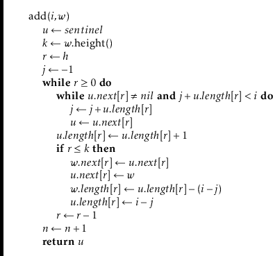
Any time the search path moves down from
.
Any time the search path moves down from
![]() with
with
![]() , we
splice
, we
splice
![]() into
into
![]() . The only extra care needed is to ensure that
the lengths of edges are updated properly. See Figure 4.6.
. The only extra care needed is to ensure that
the lengths of edges are updated properly. See Figure 4.6.
Note that, each time the search path goes down at a node,
![]() , in
, in
![]() ,
the length of the edge
,
the length of the edge
![]() increases by one, since we are adding
an element below that edge at position
increases by one, since we are adding
an element below that edge at position
![]() . Splicing the node
. Splicing the node
![]() between two nodes,
between two nodes,
![]() and
and
![]() , works as shown in Figure 4.7. While
following the search path we are already keeping track of the position,
, works as shown in Figure 4.7. While
following the search path we are already keeping track of the position,
![]() , of
, of
![]() in
in ![]() . Therefore, we know that the length of the edge from
. Therefore, we know that the length of the edge from
![]() to
to
![]() is
is
![]() . We can also deduce the length of the edge
from
. We can also deduce the length of the edge
from
![]() to
to
![]() from the length,
from the length, ![]() , of the edge from
, of the edge from
![]() to
to
![]() .
Therefore, we can splice in
.
Therefore, we can splice in
![]() and update the lengths of the edges in
constant time.
and update the lengths of the edges in
constant time.
This sounds more complicated than it is, for the code is actually quite simple:
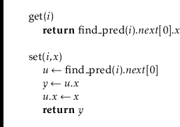
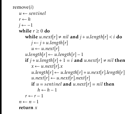
By now, the implementation of
the
![]() operation in a SkiplistList should be obvious. We follow the search path for the node at position
operation in a SkiplistList should be obvious. We follow the search path for the node at position
![]() . Each time the search path takes a step down from a node,
. Each time the search path takes a step down from a node,
![]() , at level
, at level
![]() we decrement the length of the edge leaving
we decrement the length of the edge leaving
![]() at that level. We also check if
at that level. We also check if
![]() is the element of rank
is the element of rank
![]() and, if so, splice it out of the list at that level. An example is shown in Figure 4.8.
and, if so, splice it out of the list at that level. An example is shown in Figure 4.8.
The following theorem summarizes the performance of the SkiplistList data structure:
![\includegraphics[width=\textwidth ]{figs-python/skiplist-lengths}](img1691.png)
![\includegraphics[width=\textwidth ]{figs-python/skiplist-addix}](img1720.png)
![\includegraphics[scale=0.90909]{figs-python/skiplist-lengths-splice}](img1740.png)
![\includegraphics[width=\textwidth ]{figs-python/skiplist-removei}](img1751.png)