Next: 10.3 Discussion and Exercises Up: 10. Heaps Previous: 10.1 BinaryHeap: An Implicit Contents Index
In this section, we describe the MeldableHeap, a priority Queue implementation in which the underlying structure is also a heap-ordered binary tree. However, unlike a BinaryHeap in which the underlying binary tree is completely defined by the number of elements, there are no restrictions on the shape of the binary tree that underlies a MeldableHeap; anything goes.
The
![]() and
and
![]() operations in a MeldableHeap are
implemented in terms of the
operations in a MeldableHeap are
implemented in terms of the
![]() operation. This operation
takes two heap nodes
operation. This operation
takes two heap nodes
![]() and
and
![]() and merges them, returning a heap
node that is the root of a heap that contains all elements in the subtree
rooted at
and merges them, returning a heap
node that is the root of a heap that contains all elements in the subtree
rooted at
![]() and all elements in the subtree rooted at
and all elements in the subtree rooted at
![]() .
.
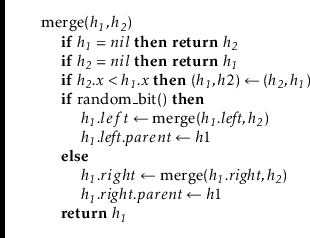
The nice thing about a
![]() operation is that it can be
defined recursively. See Figure 10.4. If either
operation is that it can be
defined recursively. See Figure 10.4. If either
![]() or
or
![]() is
is
![]() , then we are merging with an empty set, so we return
, then we are merging with an empty set, so we return
![]() or
or
![]() , respectively. Otherwise, assume
, respectively. Otherwise, assume
![]() since,
if
since,
if
![]() , then we can reverse the roles of
, then we can reverse the roles of
![]() and
and
![]() .
Then we know that the root of the merged heap will contain
.
Then we know that the root of the merged heap will contain
![]() , and
we can recursively merge
, and
we can recursively merge
![]() with
with
![]() or
or
![]() , as we wish.
This is where randomization comes in, and we toss a coin to decide
whether to merge
, as we wish.
This is where randomization comes in, and we toss a coin to decide
whether to merge
![]() with
with
![]() or
or
![]() :
:
In the next section, we show that
![]() runs in
runs in
![]() expected time, where
expected time, where
![]() is the total number of elements in
is the total number of elements in
![]() and
and
![]() .
.
With access to a
![]() operation, the
operation, the
![]() operation is easy. We create a new node
operation is easy. We create a new node
![]() containing
containing
![]() and then merge
and then merge
![]() with the root of our heap:
with the root of our heap:
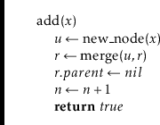
This takes
![]() expected time.
expected time.
The
![]() operation is similarly easy. The node we want to remove
is the root, so we just merge its two children and make the result the root:
operation is similarly easy. The node we want to remove
is the root, so we just merge its two children and make the result the root:
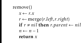
Again, this takes
![]() expected time.
expected time.
Additionally, a MeldableHeap can implement many other operations in
![]() expected time, including:
expected time, including:
The analysis of
![]() is based on the analysis of a random walk
in a binary tree. A random walk in a binary tree starts at the
root of the tree. At each step in the random walk, a coin is tossed and,
depending on the result of this coin toss, the walk proceeds to the left
or to the right child of the current node. The walk ends when it falls
off the tree (the current node becomes
is based on the analysis of a random walk
in a binary tree. A random walk in a binary tree starts at the
root of the tree. At each step in the random walk, a coin is tossed and,
depending on the result of this coin toss, the walk proceeds to the left
or to the right child of the current node. The walk ends when it falls
off the tree (the current node becomes
![]() ).
).
The following lemma is somewhat remarkable because it does not depend at all on the shape of the binary tree:
Let
![]() denote the size of the root's left subtree, so that
denote the size of the root's left subtree, so that
![]() is the size of the root's right subtree. Starting at
the root, the walk takes one step and then continues in a subtree of
size
is the size of the root's right subtree. Starting at
the root, the walk takes one step and then continues in a subtree of
size
![]() or
or
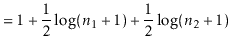
![]() . By our inductive hypothesis, the expected
length of the walk is then
. By our inductive hypothesis, the expected
length of the walk is then
![$\displaystyle \mathrm{E}[W] = 1 + \frac{1}{2}\log (\ensuremath{\ensuremath{\ens...
...{1}{2}\log (\ensuremath{\ensuremath{\ensuremath{\mathit{n}}}}_2+1) \enspace ,
$](img3988.png)
 |
||
We make a quick digression to note that, for readers who know a little about information theory, the proof of Lemma 10.1 can be stated in terms of entropy.
With this result on random walks, we can now easily prove that the
running time of the
![]() operation is
operation is
![]() .
.
The following theorem summarizes the performance of a MeldableHeap:
![\includegraphics[width=\textwidth ]{figs-python/meldable-merge}](img3944.png)