Next: 13.2 XFastTrie: Searching in Up: 13. Data Structures for Previous: 13. Data Structures for Contents Index
A BinaryTrie encodes a set of
![]() bit integers in a binary tree.
All leaves in the tree have depth
bit integers in a binary tree.
All leaves in the tree have depth
![]() and each integer is encoded as a
root-to-leaf path. The path for the integer
and each integer is encoded as a
root-to-leaf path. The path for the integer
![]() turns left at level
turns left at level
![]() if the
if the
![]() th most significant bit of
th most significant bit of
![]() is a 0 and turns right if it
is a 1. Figure 13.1 shows an example for the case
is a 0 and turns right if it
is a 1. Figure 13.1 shows an example for the case
![]() ,
in which the trie stores the integers 3(0011), 9(1001), 12(1100),
and 13(1101).
,
in which the trie stores the integers 3(0011), 9(1001), 12(1100),
and 13(1101).
Because the search path
for a value
![]() depends on the bits of
depends on the bits of
![]() , it will
be helpful to name the children of a node,
, it will
be helpful to name the children of a node,
![]() ,
,
![]() (
(
![]() )
and
)
and
![]() (
(
![]() ). These child pointers will actually serve
double-duty. Since the leaves in a binary trie have no children, the
pointers are used to string the leaves together into a doubly-linked list.
For a leaf in the binary trie
). These child pointers will actually serve
double-duty. Since the leaves in a binary trie have no children, the
pointers are used to string the leaves together into a doubly-linked list.
For a leaf in the binary trie
![]() (
(
![]() ) is the node that
comes before
) is the node that
comes before
![]() in the list and
in the list and
![]() (
(
![]() ) is the node that
follows
) is the node that
follows
![]() in the list. A special node,
in the list. A special node,
![]() , is used both before
the first node and after the last node in the list (see Section 3.2).
, is used both before
the first node and after the last node in the list (see Section 3.2).
Each node,
![]() , also contains an additional pointer
, also contains an additional pointer
![]() . If
. If
![]() 's
left child is missing, then
's
left child is missing, then
![]() points to the smallest leaf in
points to the smallest leaf in
![]() 's subtree. If
's subtree. If
![]() 's right child is missing, then
's right child is missing, then
![]() points
to the largest leaf in
points
to the largest leaf in
![]() 's subtree. An example of a BinaryTrie,
showing
's subtree. An example of a BinaryTrie,
showing
![]() pointers and the doubly-linked list at the leaves, is
shown in Figure 13.2.
pointers and the doubly-linked list at the leaves, is
shown in Figure 13.2.
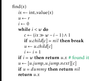
The
![]() operation in a BinaryTrie is fairly straightforward.
We try to follow the search path for
operation in a BinaryTrie is fairly straightforward.
We try to follow the search path for
![]() in the trie. If we reach a leaf,
then we have found
in the trie. If we reach a leaf,
then we have found
![]() . If we reach a node
. If we reach a node
![]() where we cannot proceed
(because
where we cannot proceed
(because
![]() is missing a child), then we follow
is missing a child), then we follow
![]() , which takes us
either to the smallest leaf larger than
, which takes us
either to the smallest leaf larger than
![]() or the largest leaf smaller than
or the largest leaf smaller than
![]() . Which of these two cases occurs depends on whether
. Which of these two cases occurs depends on whether
![]() is missing
its left or right child, respectively. In the former case (
is missing
its left or right child, respectively. In the former case (
![]() is missing
its left child), we have found the node we want. In the latter case (
is missing
its left child), we have found the node we want. In the latter case (
![]() is missing its right child), we can use the linked list to reach the node
we want. Each of these cases is illustrated in Figure 13.3.
is missing its right child), we can use the linked list to reach the node
we want. Each of these cases is illustrated in Figure 13.3.
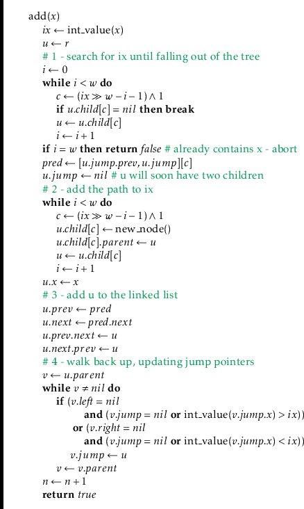
The
![]() operation in a BinaryTrie is also fairly straightforward,
but has a lot of work to do:
operation in a BinaryTrie is also fairly straightforward,
but has a lot of work to do:
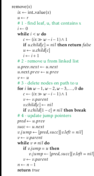
The
![]() operation undoes the work of
operation undoes the work of
![]() . Like
. Like
![]() ,
it has a lot of work to do:
,
it has a lot of work to do:
![\includegraphics[width=\textwidth ]{figs-python/binarytrie-ex-1}](img4915.png)
![\includegraphics[width=\textwidth ]{figs-python/binarytrie-ex-2}](img4939.png)
![\includegraphics[width=\textwidth ]{figs-python/binarytrie-ex-3}](img4953.png)
![\includegraphics[width=\textwidth ]{figs-python/binarytrie-add}](img4973.png)
![\includegraphics[scale=0.90909]{figs-python/binarytrie-remove}](img4992.png)