Next: 1.4 The Model of Up: 1. Introduction Previous: 1.2 Interfaces Contents Index
In this section, we review some mathematical notations and tools used throughout this book, including logarithms, big-Oh notation, and probability theory. This review will be brief and is not intended as an introduction. Readers who feel they are missing this background are encouraged to read, and do exercises from, the appropriate sections of the very good (and free) textbook on mathematics for computer science [50].
The expression ![]() denotes the number
denotes the number ![]() raised to the power of
raised to the power of ![]() .
If
.
If ![]() is a positive integer, then this is just the value of
is a positive integer, then this is just the value of ![]() multiplied by itself
multiplied by itself ![]() times:
times:

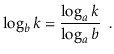
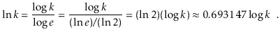
In this book, the expression ![]() denotes the base-
denotes the base-![]() logarithm
of
logarithm
of ![]() . That is, the unique value
. That is, the unique value ![]() that satisfies
that satisfies
An informal, but useful, way to think about logarithms is to think
of ![]() as the number of times we have to divide
as the number of times we have to divide ![]() by
by ![]() before the result is less than or equal to 1. For example, when one
does binary search, each comparison reduces the number of possible
answers by a factor of 2. This is repeated until there is at most one
possible answer. Therefore, the number of comparison done by binary
search when there are initially at most
before the result is less than or equal to 1. For example, when one
does binary search, each comparison reduces the number of possible
answers by a factor of 2. This is repeated until there is at most one
possible answer. Therefore, the number of comparison done by binary
search when there are initially at most ![]() possible answers is at
most
possible answers is at
most
![]() .
.
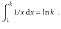
Another logarithm that comes up several times in this book is the
natural logarithm. Here we use the notation ![]() to denote
to denote
![]() , where
, where ![]() -- Euler's constant -- is given by
-- Euler's constant -- is given by
In one or two places in this book, the factorial function is used.
For a non-negative integer ![]() , the notation
, the notation ![]() (pronounced ``
(pronounced ``![]() factorial'') is defined to mean
factorial'') is defined to mean
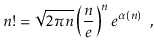
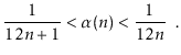
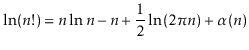
The quantity ![]() can be approximated using Stirling's Approximation:
can be approximated using Stirling's Approximation:
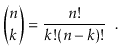
Related to the factorial function are the binomial coefficients.
For a non-negative integer ![]() and an integer
and an integer
![]() ,
the notation
,
the notation
![]() denotes:
denotes:
When analyzing data structures in this book, we want to talk about
the running times of various operations. The exact running times will,
of course, vary from computer to computer and even from run to run on an
individual computer. When we talk about the running time of an operation
we are referring to the number of computer instructions performed during
the operation. Even for simple code, this quantity can be difficult to
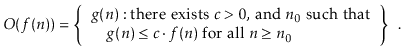
compute exactly. Therefore, instead of analyzing running times exactly,
we will use the so-called big-Oh notation: For a function ![]() ,
,
![]() denotes a set of functions,
denotes a set of functions,
We generally use asymptotic notation to simplify functions. For example,
in place of
![]() we can write
we can write
![]() .
This is proven as follows:
.
This is proven as follows:
A number of useful shortcuts can be applied when using asymptotic notation. First:
Continuing in a long and distinguished tradition, we will abuse this
notation by writing things like
![]() when what we really
mean is
when what we really
mean is
![]() . We will also make statements like ``the
running time of this operation is
. We will also make statements like ``the
running time of this operation is ![]() '' when this statement should
be ``the running time of this operation is a member of
'' when this statement should
be ``the running time of this operation is a member of ![]() .''
These shortcuts are mainly to avoid awkward language and to make it
easier to use asymptotic notation within strings of equations.
.''
These shortcuts are mainly to avoid awkward language and to make it
easier to use asymptotic notation within strings of equations.
A particularly strange example of this occurs when we write statements like
The expression ![]() also brings up another issue. Since there is
no variable in this expression, it may not be clear which variable is
getting arbitrarily large. Without context, there is no way to tell.
In the example above, since the only variable in the rest of the equation
is
also brings up another issue. Since there is
no variable in this expression, it may not be clear which variable is
getting arbitrarily large. Without context, there is no way to tell.
In the example above, since the only variable in the rest of the equation
is ![]() , we can assume that this should be read as
, we can assume that this should be read as
![]() , where
, where ![]() .
.
Big-Oh notation is not new or unique to computer science. It was used by the number theorist Paul Bachmann as early as 1894, and is immensely useful for describing the running times of computer algorithms. Consider the following piece of code:
  void  snippet() {
    for (int i = 0; i < n; i++)
      a[i] = i;
  }
One execution of this method involves
Big-Oh notation allows us to reason at a much higher level, making
it possible to analyze more complicated functions. If two algorithms
have the same big-Oh running time, then we won't know which is faster,
and there may not be a clear winner. One may be faster on one machine,
and the other may be faster on a different machine. However, if the
two algorithms have demonstrably different big-Oh running times, then
we can be certain that the one with the smaller running time will be
faster for large enough values of
![]() .
.
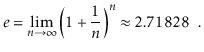
An example of how big-Oh notation allows us to compare two different
functions is shown in Figure 1.5, which compares the rate
of growth of
![]() versus
versus
![]() . It might be
that
. It might be
that ![]() is the running time of a complicated linear time algorithm
while
is the running time of a complicated linear time algorithm
while ![]() is the running time of a considerably simpler algorithm
based on the divide-and-conquer paradigm. This illustrates that,
although
is the running time of a considerably simpler algorithm
based on the divide-and-conquer paradigm. This illustrates that,
although
![]() is greater than
is greater than ![]() for small values of
for small values of
![]() ,
the opposite is true for large values of
,
the opposite is true for large values of
![]() . Eventually
. Eventually
![]() wins out, by an increasingly wide margin. Analysis using big-Oh notation
told us that this would happen, since
wins out, by an increasingly wide margin. Analysis using big-Oh notation
told us that this would happen, since
![]() .
.
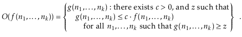
In a few cases, we will use asymptotic notation on functions with more than one variable. There seems to be no standard for this, but for our purposes, the following definition is sufficient:
Some of the data structures presented in this book are randomized; they make random choices that are independent of the data being stored in them or the operations being performed on them. For this reason, performing the same set of operations more than once using these structures could result in different running times. When analyzing these data structures we are interested in their average or expected running times.
Formally, the running time of an operation on a randomized data structure
is a random variable, and we want to study its expected value.
For
a discrete random variable ![]() taking on values in some countable
universe
taking on values in some countable
universe ![]() , the expected value of
, the expected value of ![]() , denoted by
, denoted by
![]() , is given
by the formula
, is given
by the formula
![$\displaystyle \mathrm{E}[X] = \sum_{x\in U} x\cdot\Pr\{X=x\} \enspace .
$](img434.png)
One of the most important properties of expected values is linearity
of expectation.
For any two random variables ![]() and
and ![]() ,
,
![$\displaystyle \mathrm{E}\left[\sum_{i=1}^k X_k\right] = \sum_{i=1}^k \mathrm{E}[X_i] \enspace .
$](img441.png)
A useful trick, that we will use repeatedly, is defining indicator
random variables.
These binary variables are useful when we want to
count something and are best illustrated by an example. Suppose we toss
a fair coin ![]() times and we want to know the expected number of times
the coin turns up as heads.
Intuitively, we know the answer is
times and we want to know the expected number of times
the coin turns up as heads.
Intuitively, we know the answer is ![]() ,
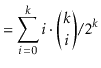
but if we try to prove it using the definition of expected value, we get
,
but if we try to prove it using the definition of expected value, we get
 |
||
 |
||
 |
||
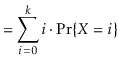
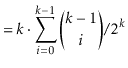
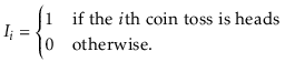
Using indicator variables and linearity of expectation makes things
much easier. For each
![]() , define the indicator
random variable
, define the indicator
random variable
![$\displaystyle = \mathrm{E}\left[\sum_{i=1}^k I_i\right]$](img457.png) |
||
![$\displaystyle = \sum_{i=1}^k \mathrm{E}[I_i]$](img458.png) |
||
 |
||
opendatastructures.org