9.2 RedBlackTree: A Simulated 2-4 Tree

A red-black tree is a binary search tree in which each node, $\ensuremath{\ensuremath{\mathit{u}}}$, has a colour which is either red or black. Red is represented by the value 0 and black by the value $1$.

Before and after any operation on a red-black tree, the following two properties are satisfied. Each property is defined both in terms of the colours red and black, and in terms of the numeric values 0 and 1.

Property 9..3 (black-height)   There are the same number of black nodes on every root to leaf path. (The sum of the colours on any root to leaf path is the same.)

Property 9..4 (no-red-edge)   No two red nodes are adjacent. (For any node $\ensuremath{\ensuremath{\mathit{u}}}$, except the root, $\ensuremath{\ensuremath{\ensuremath{\mathit{u}}.\ensuremath{\mathit{colour}}}}... ...h{\mathit{u}}.\ensuremath{\mathit{parent}}.\ensuremath{\mathit{colour}}}} \ge 1$.)

Notice that we can always colour the root, $\ensuremath{\ensuremath{\mathit{r}}}$, of a red-black tree black without violating either of these two properties, so we will assume that the root is black, and the algorithms for updating a red-black tree will maintain this. Another trick that simplifies red-black trees is to treat the external nodes (represented by $\ensuremath{\ensuremath{\mathit{nil}}}$) as black nodes. This way, every real node, $\ensuremath{\ensuremath{\mathit{u}}}$, of a red-black tree has exactly two children, each with a well-defined colour. An example of a red-black tree is shown in Figure 9.4.

Figure 9.4: An example of a red-black tree with black-height 3. External ( $\ensuremath{\ensuremath{\mathit{nil}}}$) nodes are drawn as squares.

9.2.1 Red-Black Trees and 2-4 Trees

At first it might seem surprising that a red-black tree can be efficiently updated to maintain the black-height and no-red-edge properties, and it seems unusual to even consider these as useful properties. However, red-black trees were designed to be an efficient simulation of 2-4 trees as binary trees.

Refer to Figure 9.5. Consider any red-black tree, $T$, having $\ensuremath{\ensuremath{\mathit{n}}}$ nodes and perform the following transformation: Remove each red node $\ensuremath{\ensuremath{\mathit{u}}}$ and connect $\ensuremath{\ensuremath{\mathit{u}}}$'s two children directly to the (black) parent of $\ensuremath{\ensuremath{\mathit{u}}}$. After this transformation we are left with a tree $T'$ having only black nodes.

Figure 9.5: Every red-black tree has a corresponding 2-4 tree.

Every internal node in $T'$ has two, three, or four children: A black node that started out with two black children will still have two black children after this transformation. A black node that started out with one red and one black child will have three children after this transformation. A black node that started out with two red children will have four children after this transformation. Furthermore, the black-height property now guarantees that every root-to-leaf path in $T'$ has the same length. In other words, $T'$ is a 2-4 tree!

The 2-4 tree $T'$ has $\ensuremath{\ensuremath{\ensuremath{\mathit{n}}}}+1$ leaves that correspond to the $\ensuremath{\ensuremath{\ensuremath{\mathit{n}}}}+1$ external nodes of the red-black tree. Therefore, this tree has height at most $\log (\ensuremath{\ensuremath{\ensuremath{\mathit{n}}}}+1)$. Now, every root to leaf path in the 2-4 tree corresponds to a path from the root of the red-black tree $T$ to an external node. The first and last node in this path are black and at most one out of every two internal nodes is red, so this path has at most $\log(\ensuremath{\ensuremath{\ensuremath{\mathit{n}}}}+1)$ black nodes and at most $\log(\ensuremath{\ensuremath{\ensuremath{\mathit{n}}}}+1)-1$ red nodes. Therefore, the longest path from the root to any internal node in $T$ is at most

$$2\log(\ensuremath{\ensuremath{\ensuremath{\mathit{n}}}}+1) -2 \le 2\log \ensuremath{\ensuremath{\ensuremath{\mathit{n}}}} \enspace ,$$

for any $\ensuremath{\ensuremath{\ensuremath{\mathit{n}}}}\ge 1$. This proves the most important property of red-black trees:

Lemma 9..2   The height of red-black tree with $\ensuremath{\ensuremath{\mathit{n}}}$ nodes is at most $2\log \ensuremath{\ensuremath{\ensuremath{\mathit{n}}}}$.

Now that we have seen the relationship between 2-4 trees and red-black trees, it is not hard to believe that we can efficiently maintain a red-black tree while adding and removing elements.

We have already seen that adding an element in a BinarySearchTree can be done by adding a new leaf. Therefore, to implement $\ensuremath{\mathrm{add}(\ensuremath{\mathit{x}})}$ in a red-black tree we need a method of simulating splitting a node with five children in a 2-4 tree. A 2-4 tree node with five children is represented by a black node that has two red children, one of which also has a red child. We can ``split'' this node by colouring it red and colouring its two children black. An example of this is shown in Figure 9.6.

Figure 9.6: Simulating a 2-4 tree split operation during an addition in a red-black tree. (This simulates the 2-4 tree addition shown in Figure 9.2.)

Similarly, implementing $\ensuremath{\mathrm{remove}(\ensuremath{\mathit{x}})}$ requires a method of merging two nodes and borrowing a child from a sibling. Merging two nodes is the inverse of a split (shown in Figure 9.6), and involves colouring two (black) siblings red and colouring their (red) parent black. Borrowing from a sibling is the most complicated of the procedures and involves both rotations and recolouring nodes.

Of course, during all of this we must still maintain the no-red-edge property and the black-height property. While it is no longer surprising that this can be done, there are a large number of cases that have to be considered if we try to do a direct simulation of a 2-4 tree by a red-black tree. At some point, it just becomes simpler to disregard the underlying 2-4 tree and work directly towards maintaining the properties of the red-black tree.

9.2.2 Left-Leaning Red-Black Trees

No single definition of red-black trees exists. Rather, there is a family of structures that manage to maintain the black-height and no-red-edge properties during $\ensuremath{\mathrm{add}(\ensuremath{\mathit{x}})}$ and $\ensuremath{\mathrm{remove}(\ensuremath{\mathit{x}})}$ operations. Different structures do this in different ways. Here, we implement a data structure that we call a RedBlackTree. This structure implements a particular variant of red-black trees that satisfies an additional property:

Property 9..5 (left-leaning)   At any node $\ensuremath{\ensuremath{\mathit{u}}}$, if $\ensuremath{\ensuremath{\mathit{u}}.\ensuremath{\mathit{left}}}$ is black, then $\ensuremath{\ensuremath{\mathit{u}}.\ensuremath{\mathit{right}}}$ is black.

Note that the red-black tree shown in Figure 9.4 does not satisfy the left-leaning property; it is violated by the parent of the red node in the rightmost path.

The reason for maintaining the left-leaning property is that it reduces the number of cases encountered when updating the tree during $\ensuremath{\mathrm{add}(\ensuremath{\mathit{x}})}$ and $\ensuremath{\mathrm{remove}(\ensuremath{\mathit{x}})}$ operations. In terms of 2-4 trees, it implies that every 2-4 tree has a unique representation: A node of degree two becomes a black node with two black children. A node of degree three becomes a black node whose left child is red and whose right child is black. A node of degree four becomes a black node with two red children.

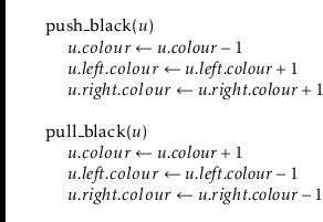
Before we describe the implementation of $\ensuremath{\mathrm{add}(\ensuremath{\mathit{x}})}$ and $\ensuremath{\mathrm{remove}(\ensuremath{\mathit{x}})}$ in detail, we first present some simple subroutines used by these methods that are illustrated in Figure 9.7. The first two subroutines are for manipulating colours while preserving the black-height property. The $\ensuremath{\mathrm{push\_black}(\ensuremath{\mathit{u}})}$ method takes as input a black node $\ensuremath{\ensuremath{\mathit{u}}}$ that has two red children and colours $\ensuremath{\ensuremath{\mathit{u}}}$ red and its two children black. The $\ensuremath{\mathrm{pull\_black}(\ensuremath{\mathit{u}})}$ method reverses this operation:

Figure 9.7: Flips, pulls and pushes

The $\ensuremath{\mathrm{flip\_left}(\ensuremath{\mathit{u}})}$ method swaps the colours of $\ensuremath{\ensuremath{\mathit{u}}}$ and $\ensuremath{\ensuremath{\mathit{u}}.\ensuremath{\mathit{right}}}$ and then performs a left rotation at $\ensuremath{\ensuremath{\mathit{u}}}$. This method reverses the colours of these two nodes as well as their parent-child relationship:

The $\ensuremath{\mathrm{flip\_left}(\ensuremath{\mathit{u}})}$ operation is especially useful in restoring the left-leaning property at a node $\ensuremath{\ensuremath{\mathit{u}}}$ that violates it (because $\ensuremath{\ensuremath{\mathit{u}}.\ensuremath{\mathit{left}}}$ is black and $\ensuremath{\ensuremath{\mathit{u}}.\ensuremath{\mathit{right}}}$ is red). In this special case, we can be assured that this operation preserves both the black-height and no-red-edge properties. The $\ensuremath{\mathrm{flip\_right}(\ensuremath{\mathit{u}})}$ operation is symmetric with $\ensuremath{\mathrm{flip\_left}(\ensuremath{\mathit{u}})}$, when the roles of left and right are reversed.

9.2.3 Addition

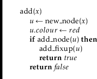
To implement $\ensuremath{\mathrm{add}(\ensuremath{\mathit{x}})}$ in a RedBlackTree, we perform a standard BinarySearchTree insertion to add a new leaf, $\ensuremath{\ensuremath{\mathit{u}}}$, with $\ensuremath{\ensuremath{\ensuremath{\mathit{u}}.\ensuremath{\mathit{x}}}}=\ensuremath{\ensuremath{\ensuremath{\mathit{x}}}}$ and set $\ensuremath{\ensuremath{\ensuremath{\mathit{u}}.\ensuremath{\mathit{colour}}}}=\ensuremath{\ensuremath{\ensuremath{\mathit{red}}}}$. Note that this does not change the black height of any node, so it does not violate the black-height property. It may, however, violate the left-leaning property (if $\ensuremath{\ensuremath{\mathit{u}}}$ is the right child of its parent), and it may violate the no-red-edge property (if $\ensuremath{\ensuremath{\mathit{u}}}$'s parent is $\ensuremath{\ensuremath{\mathit{red}}}$). To restore these properties, we call the method $\ensuremath{\mathrm{add\_fixup}(\ensuremath{\mathit{u}})}$.

Illustrated in Figure 9.8, the $\ensuremath{\mathrm{add\_fixup}(\ensuremath{\mathit{u}})}$ method takes as input a node $\ensuremath{\ensuremath{\mathit{u}}}$ whose colour is red and which may violate the no-red-edge property and/or the left-leaning property. The following discussion is probably impossible to follow without referring to Figure 9.8 or recreating it on a piece of paper. Indeed, the reader may wish to study this figure before continuing.

Figure 9.8: A single round in the process of fixing Property 2 after an insertion.

If $\ensuremath{\ensuremath{\mathit{u}}}$ is the root of the tree, then we can colour $\ensuremath{\ensuremath{\mathit{u}}}$ black to restore both properties. If $\ensuremath{\ensuremath{\mathit{u}}}$'s sibling is also red, then $\ensuremath{\ensuremath{\mathit{u}}}$'s parent must be black, so both the left-leaning and no-red-edge properties already hold.

Otherwise, we first determine if $\ensuremath{\ensuremath{\mathit{u}}}$'s parent, $\ensuremath{\ensuremath{\mathit{w}}}$, violates the left-leaning property and, if so, perform a $\ensuremath{\mathrm{flip\_left}(\ensuremath{\mathit{w}})}$ operation and set $\ensuremath{\ensuremath{\ensuremath{\mathit{u}}}}=\ensuremath{\ensuremath{\ensuremath{\mathit{w}}}}$. This leaves us in a well-defined state: $\ensuremath{\ensuremath{\mathit{u}}}$ is the left child of its parent, $\ensuremath{\ensuremath{\mathit{w}}}$, so $\ensuremath{\ensuremath{\mathit{w}}}$ now satisfies the left-leaning property. All that remains is to ensure the no-red-edge property at $\ensuremath{\ensuremath{\mathit{u}}}$. We only have to worry about the case in which $\ensuremath{\ensuremath{\mathit{w}}}$ is red, since otherwise $\ensuremath{\ensuremath{\mathit{u}}}$ already satisfies the no-red-edge property.

Since we are not done yet, $\ensuremath{\ensuremath{\mathit{u}}}$ is red and $\ensuremath{\ensuremath{\mathit{w}}}$ is red. The no-red-edge property (which is only violated by $\ensuremath{\ensuremath{\mathit{u}}}$ and not by $\ensuremath{\ensuremath{\mathit{w}}}$) implies that $\ensuremath{\ensuremath{\mathit{u}}}$'s grandparent $\ensuremath{\ensuremath{\mathit{g}}}$ exists and is black. If $\ensuremath{\ensuremath{\mathit{g}}}$'s right child is red, then the left-leaning property ensures that both $\ensuremath{\ensuremath{\mathit{g}}}$'s children are red, and a call to $\ensuremath{\mathrm{push\_black}(\ensuremath{\mathit{g}})}$ makes $\ensuremath{\ensuremath{\mathit{g}}}$ red and $\ensuremath{\ensuremath{\mathit{w}}}$ black. This restores the no-red-edge property at $\ensuremath{\ensuremath{\mathit{u}}}$, but may cause it to be violated at $\ensuremath{\ensuremath{\mathit{g}}}$, so the whole process starts over with $\ensuremath{\ensuremath{\ensuremath{\mathit{u}}}}=\ensuremath{\ensuremath{\ensuremath{\mathit{g}}}}$.

If $\ensuremath{\ensuremath{\mathit{g}}}$'s right child is black, then a call to $\ensuremath{\mathrm{flip\_right}(\ensuremath{\mathit{g}})}$ makes $\ensuremath{\ensuremath{\mathit{w}}}$ the (black) parent of $\ensuremath{\ensuremath{\mathit{g}}}$ and gives $\ensuremath{\ensuremath{\mathit{w}}}$ two red children, $\ensuremath{\ensuremath{\mathit{u}}}$ and $\ensuremath{\ensuremath{\mathit{g}}}$. This ensures that $\ensuremath{\ensuremath{\mathit{u}}}$ satisfies the no-red-edge property and $\ensuremath{\ensuremath{\mathit{g}}}$ satisfies the left-leaning property. In this case we can stop.

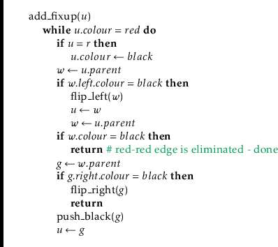
The $\ensuremath{\mathrm{insert\_fixup}(\ensuremath{\mathit{u}})}$ method takes constant time per iteration and each iteration either finishes or moves $\ensuremath{\ensuremath{\mathit{u}}}$ closer to the root. Therefore, the $\ensuremath{\mathrm{insert\_fixup}(\ensuremath{\mathit{u}})}$ method finishes after $O(\log \ensuremath{\ensuremath{\ensuremath{\mathit{n}}}})$ iterations in $O(\log \ensuremath{\ensuremath{\ensuremath{\mathit{n}}}})$ time.

9.2.4 Removal

The $\ensuremath{\mathrm{remove}(\ensuremath{\mathit{x}})}$ operation in a RedBlackTree is the most complicated to implement, and this is true of all known red-black tree variants. Just like the $\ensuremath{\mathrm{remove}(\ensuremath{\mathit{x}})}$ operation in a BinarySearchTree, this operation boils down to finding a node $\ensuremath{\ensuremath{\mathit{w}}}$ with only one child, $\ensuremath{\ensuremath{\mathit{u}}}$, and splicing $\ensuremath{\ensuremath{\mathit{w}}}$ out of the tree by having $\ensuremath{\ensuremath{\mathit{w}}.\ensuremath{\mathit{parent}}}$ adopt $\ensuremath{\ensuremath{\mathit{u}}}$.

The problem with this is that, if $\ensuremath{\ensuremath{\mathit{w}}}$ is black, then the black-height property will now be violated at $\ensuremath{\ensuremath{\mathit{w}}.\ensuremath{\mathit{parent}}}$. We may avoid this problem, temporarily, by adding $\ensuremath{\ensuremath{\mathit{w}}.\ensuremath{\mathit{colour}}}$ to $\ensuremath{\ensuremath{\mathit{u}}.\ensuremath{\mathit{colour}}}$. Of course, this introduces two other problems: (1) if $\ensuremath{\ensuremath{\mathit{u}}}$ and $\ensuremath{\ensuremath{\mathit{w}}}$ both started out black, then $\ensuremath{\ensuremath{\ensuremath{\mathit{u}}.\ensuremath{\mathit{colour}}}}+\ensuremath{\ensuremath{\ensuremath{\mathit{w}}.\ensuremath{\mathit{colour}}}}=2$ (double black), which is an invalid colour. If $\ensuremath{\ensuremath{\mathit{w}}}$ was red, then it is replaced by a black node $\ensuremath{\ensuremath{\mathit{u}}}$, which may violate the left-leaning property at $\ensuremath{\ensuremath{\ensuremath{\mathit{u}}.\ensuremath{\mathit{parent}}}}$. Both of these problems can be resolved with a call to the $\ensuremath{\mathrm{remove\_fixup}(\ensuremath{\mathit{u}})}$ method.

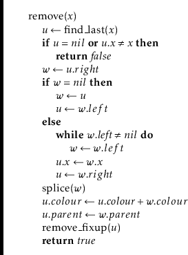
The $\ensuremath{\mathrm{remove\_fixup}(\ensuremath{\mathit{u}})}$ method takes as its input a node $\ensuremath{\ensuremath{\mathit{u}}}$ whose colour is black (1) or double-black (2). If $\ensuremath{\ensuremath{\mathit{u}}}$ is double-black, then $\ensuremath{\mathrm{remove\_fixup}(\ensuremath{\mathit{u}})}$ performs a series of rotations and recolouring operations that move the double-black node up the tree until it can be eliminated. During this process, the node $\ensuremath{\ensuremath{\mathit{u}}}$ changes until, at the end of this process, $\ensuremath{\ensuremath{\mathit{u}}}$ refers to the root of the subtree that has been changed. The root of this subtree may have changed colour. In particular, it may have gone from red to black, so the $\ensuremath{\mathrm{remove\_fixup}(\ensuremath{\mathit{u}})}$ method finishes by checking if $\ensuremath{\ensuremath{\mathit{u}}}$'s parent violates the left-leaning property and, if so, fixing it.

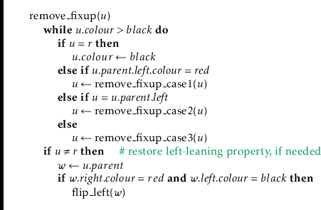
The $\ensuremath{\mathrm{remove\_fixup}(\ensuremath{\mathit{u}})}$ method is illustrated in Figure 9.9. Again, the following text will be difficult, if not impossible, to follow without referring to Figure 9.9. Each iteration of the loop in $\ensuremath{\mathrm{remove\_fixup}(\ensuremath{\mathit{u}})}$ processes the double-black node $\ensuremath{\ensuremath{\mathit{u}}}$, based on one of four cases:

Figure 9.9: A single round in the process of eliminating a double-black node after a removal.

Case 0: $\ensuremath{\ensuremath{\mathit{u}}}$ is the root. This is the easiest case to treat. We recolour $\ensuremath{\ensuremath{\mathit{u}}}$ to be black (this does not violate any of the red-black tree properties).

Case 1: $\ensuremath{\ensuremath{\mathit{u}}}$'s sibling, $\ensuremath{\ensuremath{\mathit{v}}}$, is red. In this case, $\ensuremath{\ensuremath{\mathit{u}}}$'s sibling is the left child of its parent, $\ensuremath{\ensuremath{\mathit{w}}}$ (by the left-leaning property). We perform a right-flip at $\ensuremath{\ensuremath{\mathit{w}}}$ and then proceed to the next iteration. Note that this action causes $\ensuremath{\ensuremath{\mathit{w}}}$'s parent to violate the left-leaning property and the depth of $\ensuremath{\ensuremath{\mathit{u}}}$ to increase. However, it also implies that the next iteration will be in Case 3 with $\ensuremath{\ensuremath{\mathit{w}}}$ coloured red. When examining Case 3 below, we will see that the process will stop during the next iteration.

Case 2: $\ensuremath{\ensuremath{\mathit{u}}}$'s sibling, $\ensuremath{\ensuremath{\mathit{v}}}$, is black, and $\ensuremath{\ensuremath{\mathit{u}}}$ is the left child of its parent, $\ensuremath{\ensuremath{\mathit{w}}}$. In this case, we call $\ensuremath{\mathrm{pull\_black}(\ensuremath{\mathit{w}})}$, making $\ensuremath{\ensuremath{\mathit{u}}}$ black, $\ensuremath{\ensuremath{\mathit{v}}}$ red, and darkening the colour of $\ensuremath{\ensuremath{\mathit{w}}}$ to black or double-black. At this point, $\ensuremath{\ensuremath{\mathit{w}}}$ does not satisfy the left-leaning property, so we call $\ensuremath{\mathrm{flip\_left}(\ensuremath{\mathit{w}})}$ to fix this.

At this point, $\ensuremath{\ensuremath{\mathit{w}}}$ is red and $\ensuremath{\ensuremath{\mathit{v}}}$ is the root of the subtree with which we started. We need to check if $\ensuremath{\ensuremath{\mathit{w}}}$ causes the no-red-edge property to be violated. We do this by inspecting $\ensuremath{\ensuremath{\mathit{w}}}$'s right child, $\ensuremath{\ensuremath{\mathit{q}}}$. If $\ensuremath{\ensuremath{\mathit{q}}}$ is black, then $\ensuremath{\ensuremath{\mathit{w}}}$ satisfies the no-red-edge property and we can continue the next iteration with $\ensuremath{\ensuremath{\ensuremath{\mathit{u}}}}=\ensuremath{\ensuremath{\ensuremath{\mathit{v}}}}$.

Otherwise ( $\ensuremath{\ensuremath{\mathit{q}}}$ is red), so both the no-red-edge property and the left-leaning properties are violated at $\ensuremath{\ensuremath{\mathit{q}}}$ and $\ensuremath{\ensuremath{\mathit{w}}}$, respectively. The left-leaning property is restored with a call to $\ensuremath{\mathrm{rotate\_left}(\ensuremath{\mathit{w}})}$, but the no-red-edge property is still violated. At this point, $\ensuremath{\ensuremath{\mathit{q}}}$ is the left child of $\ensuremath{\ensuremath{\mathit{v}}}$, $\ensuremath{\ensuremath{\mathit{w}}}$ is the left child of $\ensuremath{\ensuremath{\mathit{q}}}$, $\ensuremath{\ensuremath{\mathit{q}}}$ and $\ensuremath{\ensuremath{\mathit{w}}}$ are both red, and $\ensuremath{\ensuremath{\mathit{v}}}$ is black or double-black. A $\ensuremath{\mathrm{flip\_right}(\ensuremath{\mathit{v}})}$ makes $\ensuremath{\ensuremath{\mathit{q}}}$ the parent of both $\ensuremath{\ensuremath{\mathit{v}}}$ and $\ensuremath{\ensuremath{\mathit{w}}}$. Following this up by a $\ensuremath{\mathrm{push\_black}(\ensuremath{\mathit{q}})}$ makes both $\ensuremath{\ensuremath{\mathit{v}}}$ and $\ensuremath{\ensuremath{\mathit{w}}}$ black and sets the colour of $\ensuremath{\ensuremath{\mathit{q}}}$ back to the original colour of $\ensuremath{\ensuremath{\mathit{w}}}$.

At this point, the double-black node is has been eliminated and the no-red-edge and black-height properties are reestablished. Only one possible problem remains: the right child of $\ensuremath{\ensuremath{\mathit{v}}}$ may be red, in which case the left-leaning property would be violated. We check this and perform a $\ensuremath{\mathrm{flip\_left}(\ensuremath{\mathit{v}})}$ to correct it if necessary.

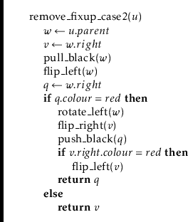
Case 3: $\ensuremath{\ensuremath{\mathit{u}}}$'s sibling is black and $\ensuremath{\ensuremath{\mathit{u}}}$ is the right child of its parent, $\ensuremath{\ensuremath{\mathit{w}}}$. This case is symmetric to Case 2 and is handled mostly the same way. The only differences come from the fact that the left-leaning property is asymmetric, so it requires different handling.

As before, we begin with a call to $\ensuremath{\mathrm{pull\_black}(\ensuremath{\mathit{w}})}$, which makes $\ensuremath{\ensuremath{\mathit{v}}}$ red and $\ensuremath{\ensuremath{\mathit{u}}}$ black. A call to $\ensuremath{\mathrm{flip\_right}(\ensuremath{\mathit{w}})}$ promotes $\ensuremath{\ensuremath{\mathit{v}}}$ to the root of the subtree. At this point $\ensuremath{\ensuremath{\mathit{w}}}$ is red, and the code branches two ways depending on the colour of $\ensuremath{\ensuremath{\mathit{w}}}$'s left child, $\ensuremath{\ensuremath{\mathit{q}}}$.

If $\ensuremath{\ensuremath{\mathit{q}}}$ is red, then the code finishes up exactly the same way as Case 2 does, but is even simpler since there is no danger of $\ensuremath{\ensuremath{\mathit{v}}}$ not satisfying the left-leaning property.

The more complicated case occurs when $\ensuremath{\ensuremath{\mathit{q}}}$ is black. In this case, we examine the colour of $\ensuremath{\ensuremath{\mathit{v}}}$'s left child. If it is red, then $\ensuremath{\ensuremath{\mathit{v}}}$ has two red children and its extra black can be pushed down with a call to $\ensuremath{\mathrm{push\_black}(\ensuremath{\mathit{v}})}$. At this point, $\ensuremath{\ensuremath{\mathit{v}}}$ now has $\ensuremath{\ensuremath{\mathit{w}}}$'s original colour, and we are done.

If $\ensuremath{\ensuremath{\mathit{v}}}$'s left child is black, then $\ensuremath{\ensuremath{\mathit{v}}}$ violates the left-leaning property, and we restore this with a call to $\ensuremath{\mathrm{flip\_left}(\ensuremath{\mathit{v}})}$. We then return the node $\ensuremath{\ensuremath{\mathit{v}}}$ so that the next iteration of $\ensuremath{\mathrm{remove\_fixup}(\ensuremath{\mathit{u}})}$ then continues with $\ensuremath{\ensuremath{\ensuremath{\mathit{u}}}}=\ensuremath{\ensuremath{\ensuremath{\mathit{v}}}}$.

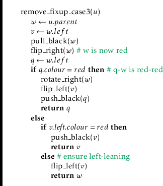
Each iteration of $\ensuremath{\mathrm{remove\_fixup}(\ensuremath{\mathit{u}})}$ takes constant time. Cases 2 and 3 either finish or move $\ensuremath{\ensuremath{\mathit{u}}}$ closer to the root of the tree. Case 0 (where $\ensuremath{\ensuremath{\mathit{u}}}$ is the root) always terminates and Case 1 leads immediately to Case 3, which also terminates. Since the height of the tree is at most $2\log \ensuremath{\ensuremath{\ensuremath{\mathit{n}}}}$, we conclude that there are at most $O(\log \ensuremath{\ensuremath{\ensuremath{\mathit{n}}}})$ iterations of $\ensuremath{\mathrm{remove\_fixup}(\ensuremath{\mathit{u}})}$, so $\ensuremath{\mathrm{remove\_fixup}(\ensuremath{\mathit{u}})}$ runs in $O(\log \ensuremath{\ensuremath{\ensuremath{\mathit{n}}}})$ time.