Next: 5.3 Hash Codes Up: 5. Hash Tables Previous: 5.1 ChainedHashTable: Hashing with Contents Index
The ChainedHashTable data structure uses an array of lists, where the
![]() th
list stores all elements
th
list stores all elements
![]() such that
such that
![]() . An alternative,
called open addressing
is to store the elements directly in an
array,
. An alternative,
called open addressing
is to store the elements directly in an
array,
![]() , with each array location in
, with each array location in
![]() storing at most one value.
This approach is taken by the LinearHashTable described in this
section. In some places, this data structure is described as open
addressing with linear probing.
storing at most one value.
This approach is taken by the LinearHashTable described in this
section. In some places, this data structure is described as open
addressing with linear probing.
The main idea behind a LinearHashTable is that we would, ideally, like
to store the element
![]() with hash value
with hash value
![]() in the table location
in the table location
![]() . If we cannot do this (because some element is already stored
there) then we try to store it at location
. If we cannot do this (because some element is already stored
there) then we try to store it at location
![]() ;
if that's not possible, then we try
;
if that's not possible, then we try
![]() ,
and so on, until we find a place for
,
and so on, until we find a place for
![]() .
.
There are three types of entries stored in
![]() :
:
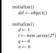
To summarize, a LinearHashTable contains an array,
![]() , that stores
data elements, and integers
, that stores
data elements, and integers
![]() and
and
![]() that keep track of the number of
data elements and non-
that keep track of the number of
data elements and non-
![]() values of
values of
![]() , respectively. Because many
hash functions only work for table sizes that are a power of 2, we also
keep an integer
, respectively. Because many
hash functions only work for table sizes that are a power of 2, we also
keep an integer
![]() and maintain the invariant that
and maintain the invariant that
![]() .
.
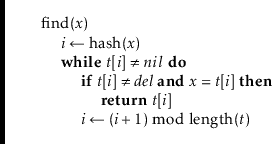
The
![]() operation in a LinearHashTable is simple. We start
at array entry
operation in a LinearHashTable is simple. We start
at array entry
![]() where
where
![]() and search entries
and search entries
![]() ,
,
![]() ,
,
![]() , and so on,
until we find an index
, and so on,
until we find an index
![]() such that, either,
such that, either,
![]() , or
, or
![]() .
In the former case we return
.
In the former case we return
![]() . In the latter case, we conclude
that
. In the latter case, we conclude
that
![]() is not contained in the hash table and return
is not contained in the hash table and return
![]() .
.
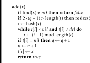
The
![]() operation is also fairly easy to implement. After checking
that
operation is also fairly easy to implement. After checking
that
![]() is not already stored in the table (using
is not already stored in the table (using
![]() ), we search
), we search
![]() ,
,
![]() ,
,
![]() ,
and so on, until we find a
,
and so on, until we find a
![]() or
or
![]() and store
and store
![]() at that location,
increment
at that location,
increment
![]() , and
, and
![]() , if appropriate.
, if appropriate.
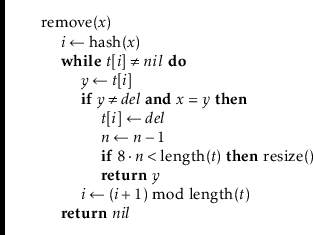
By now, the implementation of the
![]() operation should be obvious.
We search
operation should be obvious.
We search
![]() ,
,
![]() ,
,
![]() , and so on until we find an index
, and so on until we find an index
![]() such that
such that
![]() or
or
![]() . In the former case, we set
. In the former case, we set
![]() and return
and return
![]() . In the latter case we conclude that
. In the latter case we conclude that
![]() was not stored in the
table (and therefore cannot be deleted) and return
was not stored in the
table (and therefore cannot be deleted) and return
![]() .
.
The correctness of the
![]() ,
,
![]() , and
, and
![]() methods is
easy to verify, though it relies on the use of
methods is
easy to verify, though it relies on the use of
![]() values. Notice
that none of these operations ever sets a non-
values. Notice
that none of these operations ever sets a non-
![]() entry to
entry to
![]() .
Therefore, when we reach an index
.
Therefore, when we reach an index
![]() such that
such that
![]() , this is
a proof that the element,
, this is
a proof that the element,
![]() , that we are searching for is not stored
in the table;
, that we are searching for is not stored
in the table;
![]() has always been
has always been
![]() , so there is no reason that
a previous
, so there is no reason that
a previous
![]() operation would have proceeded beyond index
operation would have proceeded beyond index
![]() .
.
The
![]() method is called by
method is called by
![]() when the number of non-
when the number of non-
![]() entries exceeds
entries exceeds
![]() or by
or by
![]() when the number of
data entries is less than
when the number of
data entries is less than
![]() . The
. The
![]() method works
like the
method works
like the
![]() methods in other array-based data structures.
We find the smallest non-negative integer
methods in other array-based data structures.
We find the smallest non-negative integer
![]() such that
such that
![]() . We reallocate the array
. We reallocate the array
![]() so that it has size
so that it has size
![]() ,
and then we insert all the elements in the old version of
,
and then we insert all the elements in the old version of
![]() into the
newly-resized copy of
into the
newly-resized copy of
![]() . While doing this, we reset
. While doing this, we reset
![]() equal to
equal to
![]() since the newly-allocated
since the newly-allocated
![]() contains no
contains no
![]() values.
values.
![\begin{leftbar}
\begin{flushleft}
\hspace*{1em} \ensuremath{\mathrm{resize}()}\\...
...mathit{t}}[\ensuremath{i}] \gets \ensuremath{x}}\\
\end{flushleft}\end{leftbar}](img2194.png)
Notice that each operation,
![]() ,
,
![]() , or
, or
![]() , finishes
as soon as (or before) it discovers the first
, finishes
as soon as (or before) it discovers the first
![]() entry in
entry in
![]() .
The intuition behind the analysis of linear probing is that, since at
least half the elements in
.
The intuition behind the analysis of linear probing is that, since at
least half the elements in
![]() are equal to
are equal to
![]() , an operation should
not take long to complete because it will very quickly come across a
, an operation should
not take long to complete because it will very quickly come across a
![]() entry. We shouldn't rely too heavily on this intuition, though,
because it would lead us to (the incorrect) conclusion that the expected
number of locations in
entry. We shouldn't rely too heavily on this intuition, though,
because it would lead us to (the incorrect) conclusion that the expected
number of locations in
![]() examined by an operation is at most 2.
examined by an operation is at most 2.
For the rest of this section, we will assume that all hash values are
independently and uniformly distributed in
![]() .
This is not a realistic assumption, but it will make it possible for
us to analyze linear probing. Later in this section we will describe a
method, called tabulation hashing, that produces a hash function that is
``good enough'' for linear probing. We will also assume that all indices
into the positions of
.
This is not a realistic assumption, but it will make it possible for
us to analyze linear probing. Later in this section we will describe a
method, called tabulation hashing, that produces a hash function that is
``good enough'' for linear probing. We will also assume that all indices
into the positions of
![]() are taken modulo
are taken modulo
![]() , so that
, so that
![]() is really a shorthand for
is really a shorthand for
![]() .
.
We say that a run of length ![]() that starts at
that starts at
![]() occurs when all
the table entries
occurs when all
the table entries
![]() are non-
are non-
![]() and
and
![]() . The number of non-
. The number of non-
![]() elements of
elements of
![]() is exactly
is exactly
![]() and the
and the
![]() method ensures that, at all times,
method ensures that, at all times,
![]() . There are
. There are
![]() elements
elements
![]() that have been inserted into
that have been inserted into
![]() since the last
since the last
![]() operation.
By our assumption, each of these has a hash value,
operation.
By our assumption, each of these has a hash value,
![]() ,
that is uniform and independent of the rest. With this setup, we can
prove the main lemma required to analyze linear probing.
,
that is uniform and independent of the rest. With this setup, we can
prove the main lemma required to analyze linear probing.
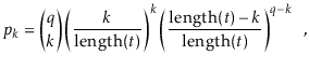
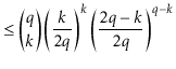
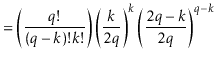
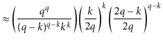
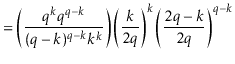
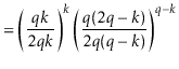
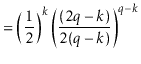
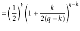
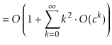
In the following derivation we will cheat a little and replace ![]() with
with
![]() . Stirling's Approximation (Section 1.3.2) shows that this
is only a factor of
. Stirling's Approximation (Section 1.3.2) shows that this
is only a factor of
![]() from the truth. This is just done to
make the derivation simpler; Exercise 5.4 asks the reader to
redo the calculation more rigorously using Stirling's Approximation in
its entirety.
from the truth. This is just done to
make the derivation simpler; Exercise 5.4 asks the reader to
redo the calculation more rigorously using Stirling's Approximation in
its entirety.
The value of ![]() is maximized when
is maximized when
![]() is minimum, and the data
structure maintains the invariant that
is minimum, and the data
structure maintains the invariant that
![]() , so
, so
 |
||||
 |
||||
 |
[Stirling's approximation] | |||
 |
||||
 |
||||
 |
||||
 |
||||
 |
Using Lemma 5.4 to prove upper-bounds on the expected
running time of
![]() ,
,
![]() , and
, and
![]() is now fairly
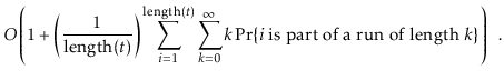
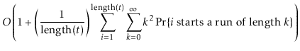
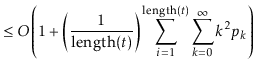
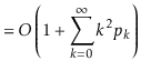
straightforward. Consider the simplest case, where we execute
is now fairly
straightforward. Consider the simplest case, where we execute
![]() for some value
for some value
![]() that has never been stored in the
LinearHashTable. In this case,
that has never been stored in the
LinearHashTable. In this case,
![]() is a random value in
is a random value in
![]() independent of the contents of
independent of the contents of
![]() . If
. If
![]() is part of a run of length
is part of a run of length ![]() , then the time it takes to execute the
, then the time it takes to execute the
![]() operation is at most
operation is at most ![]() . Thus, the expected running time
can be upper-bounded by
. Thus, the expected running time
can be upper-bounded by
 |
||
 |
||
 |
||
 |
||
If we ignore the cost of the
![]() operation, then the above
analysis gives us all we need to analyze the cost of operations on a
LinearHashTable.
operation, then the above
analysis gives us all we need to analyze the cost of operations on a
LinearHashTable.
First of all, the analysis of
![]() given above applies to the
given above applies to the
![]() operation when
operation when
![]() is not contained in the table. To analyze
the
is not contained in the table. To analyze
the
![]() operation when
operation when
![]() is contained in the table, we need only
note that this is the same as the cost of the
is contained in the table, we need only
note that this is the same as the cost of the
![]() operation that
previously added
operation that
previously added
![]() to the table. Finally, the cost of a
to the table. Finally, the cost of a
![]() operation is the same as the cost of a
operation is the same as the cost of a
![]() operation.
operation.
In summary, if we ignore the cost of calls to
![]() , all operations
on a LinearHashTable run in
, all operations
on a LinearHashTable run in ![]() expected time. Accounting for the
cost of resize can be done using the same type of amortized analysis
performed for the ArrayStack data structure in Section 2.1.
expected time. Accounting for the
cost of resize can be done using the same type of amortized analysis
performed for the ArrayStack data structure in Section 2.1.
The following theorem summarizes the performance of the LinearHashTable data structure:
Furthermore, beginning with an empty LinearHashTable, any
sequence of ![]()
![]() and
and
![]() operations results in a total
of
operations results in a total
of ![]() time spent during all calls to
time spent during all calls to
![]() .
.
While analyzing the LinearHashTable structure, we made a very strong
assumption: That for any set of elements,
![]() ,
the hash values
,
the hash values
![]() x
x
![]() are independently and
uniformly distributed over the set
are independently and
uniformly distributed over the set
![]() . One way to
achieve this is to store a giant array,
. One way to
achieve this is to store a giant array,
![]() , of length
, of length
![]() ,
where each entry is a random
,
where each entry is a random
![]() -bit integer, independent of all the
other entries. In this way, we could implement
-bit integer, independent of all the
other entries. In this way, we could implement
![]() by extracting
a
by extracting
a
![]() -bit integer from
-bit integer from
![]() :
:
![\begin{leftbar}
\begin{flushleft}
\hspace*{1em} \ensuremath{\mathrm{ideal\_hash}...
...ensuremath{\mathit{w}}-\ensuremath{\mathit{d}}]}\\
\end{flushleft}\end{leftbar}](img2324.png)
Here,
![]() , is the bitwise right shift operator, so
, is the bitwise right shift operator, so
![]() extracts the
extracts the
![]() most significant bits of
most significant bits of
![]() 's
's
![]() -bit hash code.
-bit hash code.
Unfortunately, storing an array of size
![]() is prohibitive in terms
of memory usage. The approach used by tabulation hashing is to,
instead, treat
is prohibitive in terms
of memory usage. The approach used by tabulation hashing is to,
instead, treat
![]() -bit integers as being comprised of
-bit integers as being comprised of
![]() integers, each having only
integers, each having only
![]() bits. In this way, tabulation hashing
only needs
bits. In this way, tabulation hashing
only needs
![]() arrays each of length
arrays each of length
![]() . All the entries
in these arrays are independent random
. All the entries
in these arrays are independent random
![]() -bit integers. To obtain the value
of
-bit integers. To obtain the value
of
![]() we split
we split
![]() up into
up into
![]()
![]() -bit integers
and use these as indices into these arrays. We then combine all these
values with the bitwise exclusive-or operator to obtain
-bit integers
and use these as indices into these arrays. We then combine all these
values with the bitwise exclusive-or operator to obtain
![]() .
The following code shows how this works when
.
The following code shows how this works when
![]() and
and
![]() :
:
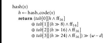
In this case,
![]() is a two-dimensional array with four columns and
is a two-dimensional array with four columns and
![]() rows.
Quantities like
rows.
Quantities like
![]() , used above, are hexadecimal numbers
whose digits have 16 possible values 0-9, which have their usual
meaning and a-f, which denote 10-15. The number
, used above, are hexadecimal numbers
whose digits have 16 possible values 0-9, which have their usual
meaning and a-f, which denote 10-15. The number
![]() .
The
.
The ![]() symbol is the bitwise and operator, so
code like
symbol is the bitwise and operator, so
code like
![]() extracts bits with index 8 through 15 of
extracts bits with index 8 through 15 of
![]() .
.
One can easily verify that, for any
![]() ,
,
![]() is uniformly
distributed over
is uniformly
distributed over
![]() . With a little work, one
can even verify that any pair of values have independent hash values.
This implies tabulation hashing could be used in place of multiplicative
hashing for the ChainedHashTable implementation.
. With a little work, one
can even verify that any pair of values have independent hash values.
This implies tabulation hashing could be used in place of multiplicative
hashing for the ChainedHashTable implementation.
However, it is not true that any set of
![]() distinct values gives a set
of
distinct values gives a set
of
![]() independent hash values. Nevertheless, when tabulation hashing is
used, the bound of Theorem 5.2 still holds. References for
this are provided at the end of this chapter.
independent hash values. Nevertheless, when tabulation hashing is
used, the bound of Theorem 5.2 still holds. References for
this are provided at the end of this chapter.