Next: 1.3 The Model of Up: 1. Introduction Previous: 1.1 Interfaces Contents
In this section, we review some mathematical notations and tools used throughout this book, including logarithms, big-Oh notation, and probability theory.
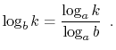
In this book, the expression ![]() denotes the base-
denotes the base-![]() logarithm
of
logarithm
of ![]() . That is, the unique value
. That is, the unique value ![]() that satisfies
that satisfies
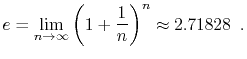
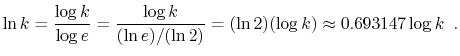
Another logarithm that comes up several times in this book is the
natural logarithm. Here we use the notation ![]() to denote
to denote
![]() , where
, where ![]() -- Euler's constant -- is given by
-- Euler's constant -- is given by
In one or two places in this book, the factorial function is used.
For a non-negative integer ![]() , the notation
, the notation ![]() (pronounced ``
(pronounced ``![]() factorial'') denotes
factorial'') denotes
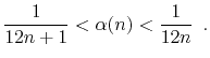
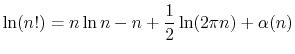
The quantity ![]() can be approximated using Stirling's Approximation:
can be approximated using Stirling's Approximation:
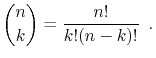
Related to the factorial function are the binomial coefficients.
For a non-negative integer ![]() and an integer
and an integer
![]() ,
the notation
,
the notation
![]() denotes:
denotes:
When analyzing data structures in this book, we will want to talk about
the running times of various operations. The exact running times will,
of course, vary from computer to computer and even from run to run on
an individual computer. Therefore, instead of analyzing running times
exactly, we will use the so-called big-Oh notation: For a
function ![]() ,
, ![]() denotes a set of functions,
denotes a set of functions,
We generally use asymptotic notation to simplify functions. For example,
in place of
![]() we can write, simply,
we can write, simply,
![]() .
This is proven as follows:
.
This is proven as follows:
There are a number of useful shortcuts when using asymptotic notation. First:
Continuing in a long and distinguished tradition,
we will abuse this notation by writing things
like
![]() when what we really mean is
when what we really mean is
![]() .
We will also make statements like ``the running time of this operation
is
.
We will also make statements like ``the running time of this operation
is ![]() '' when this statement should be ``the running time of
this operation is a member of
'' when this statement should be ``the running time of
this operation is a member of ![]() .'' These shortcuts are mainly
to avoid awkward language and to make it easier to use asymptotic
notation within strings of equations.
.'' These shortcuts are mainly
to avoid awkward language and to make it easier to use asymptotic
notation within strings of equations.
A particularly strange example of this comes when we write statements like
The expression ![]() also brings up another issue. Since there is
no variable in this expression, it may not be clear what variable is
getting arbitrarily large. Without context, there is no way to tell.
In the example above, since the only variable in the rest of the equation
is
also brings up another issue. Since there is
no variable in this expression, it may not be clear what variable is
getting arbitrarily large. Without context, there is no way to tell.
In the example above, since the only variable in the rest of the equation
is ![]() , we can assume that this should be read as
, we can assume that this should be read as
![]() ,
where
,
where ![]() .
.
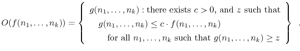
In a few cases, we will use asymptotic notation on functions with more than one variable. There seems to be no standard for this, but for our purposes, the following definition is sufficient:
Some of the data structures presented in this book are randomized; they make random choices that are independent of the data being stored in them or the operations being performed on them. For this reason, performing the same set of operations more than once using these structures could result in different running times. When analyzing these data structures we are interested in their average or expected running times.
Formally, the running time of an operation on a randomized data structure
is a random variable and we want to study its expected value. For
a discrete random variable ![]() taking on values in some countable universe
taking on values in some countable universe
![]() , the expected value of
, the expected value of ![]() , denoted by
, denoted by
![]() is given the by the formula
is given the by the formula
![$\displaystyle \mathrm{E}[X] = \sum_{x\in U} x\cdot\Pr\{X=x\} \enspace .
$](img143.png)
One of the most important properties of expected values is linearity
of expectation: For any two random variables ![]() and
and ![]() ,
,
![$\displaystyle \mathrm{E}\left[\sum_{i=1}^k X_k\right] = \sum_{i=1}^k \mathrm{E}[X_i] \enspace .
$](img149.png)
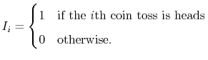
A useful trick, that we will use repeatedly, is that of defining
indicator random variables. These binary variables are useful
when we want to count something and are best illustrated by an example.
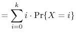
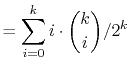
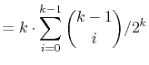
Suppose we toss a fair coin ![]() times and we want to know the expected
number of times the coin comes up heads. Intuitively, we know the answer
is
times and we want to know the expected
number of times the coin comes up heads. Intuitively, we know the answer
is ![]() , but if we try to prove it using the definition of expected
value, we get
, but if we try to prove it using the definition of expected
value, we get
 |
||
 |
||
 |
||
Using indicator variables and linearity of expectation makes things much easier: For each
![]() , define the indicator random variable
, define the indicator random variable
![$\displaystyle = \mathrm{E}\left[\sum_{i=1}^k I_i\right]$](img163.png) |
||
![$\displaystyle = \sum_{i=1}^k \mathrm{E}[I_i]$](img164.png) |
||
 |
||
opendatastructures.org