4.1 The Basic Structure

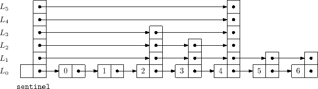
Conceptually, a skiplist is a sequence of singly-linked lists $L_0,\ldots,L_h$, where each $L_r$ contains a subset of the items in $L_{r-1}$. We start with the input list $L_0$ that contains $\mathtt{n}$ items and construct $L_1$ from $L_0$, $L_2$ from $L_1$, and so on. The items in $L_r$ are obtained by tossing a coin for each element, $\mathtt{x}$, in $L_{r-1}$ and including $\mathtt{x}$ in $L_r$ if the coin comes up heads. This process ends when we create a list $L_r$ that is empty. An example of a skiplist is shown in Figure 4.1.

Figure 4.1: A skiplist containing seven elements.

For an element, $\mathtt{x}$, in a skiplist, we call the height of $\mathtt{x}$ the largest value $r$ such that $\mathtt{x}$ appears in $L_r$. Thus, for example, elements that only appear in $L_0$ have height 0. Notice that the height of $\mathtt{x}$ corresponds to the following experiment: Toss a coin repeatedly until the first time it comes up tails. How many times did it come up heads? The answer, not surprisingly, is that the expected height of a node is 1. (We expect to toss the coin twice before getting tails, but we don't count the last toss.) The height of a skiplist is the height of its tallest node.

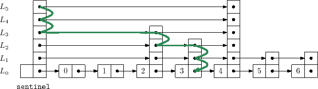
At the head of every list is a special node, called the sentinel, that acts as a dummy node for the list. The key property of skiplists is that there is a short path, called the search path, from the sentinel in $L_h$ to every node in $L_0$. Remembering how to construct a search path for a node, $\mathtt{u}$, is easy (see Figure 4.2) : Start at the top left corner of your skiplist (the sentinel in $L_h$) and always go right unless that would overshoot $\mathtt{u}$, in which case you should take a step down into the list below.

More precisely, to construct the search path for the node $\mathtt{u}$ in $L_0$ we start at the sentinel, $\mathtt{w}$, in $L_h$. Next, we examine $\mathtt{w.next}$. If $\mathtt{w.next}$ contains an item that appears before $\mathtt{u}$ in $L_0$, then we set $\ensuremath{\mathtt{w}}=\ensuremath{\mathtt{w.next}}$. Otherwise, we move down and continue the search at the occurrence of $\mathtt{w}$ in the list $L_{h-1}$. We continue this way until we reach the predecessor of $\mathtt{u}$ in $L_0$.

Figure 4.2: The search path for the node containing $4$ in a skiplist.

The following result, which we will prove in Section 4.4, shows that the search path is quite short:

Lemma 4..1   The expected length of the search path for any node, $\mathtt{u}$, in $L_0$ is at most $2\log \ensuremath{\mathtt{n}} + O(1) = O(\log \ensuremath{\mathtt{n}})$.

A space-efficient way to implement a Skiplist is to define a Node, $\mathtt{u}$, as consisting of a data value, $\mathtt{x}$, and an array, $\mathtt{next}$, of pointers, where $\mathtt{u.next[i]}$ points to $\mathtt{u}$'s successor in the list $L_{\ensuremath{\mathtt{i}}}$. In this way, the data, $\mathtt{x}$, in a node is referenced only once, even though $\mathtt{x}$ may appear in several lists.

    class Node<T> {
        T x;
        Node<T>[] next;
        Node(T ix, int h) {
            x = ix;
            next = (Node<T>[])Array.newInstance(Node.class, h+1);
        }
        int height() {
            return next.length - 1;
        }
    }

The next two sections of this chapter discuss two different applications of skiplists. In each of these applications, $L_0$ stores the main structure (a list of elements or a sorted set of elements). The primary difference between these structures is in how a search path is navigated; in particular, they differ in how they decide if a search path should go down into $L_{r-1}$ or go right within $L_r$.