Next: 2.7 Discussion and Exercises Up: 2. Array-Based Lists Previous: 2.5 : Building a Contents
One of the drawbacks of all previous data structures in this chapter
is that, because they store their data in one or two arrays, and they
avoid resizing these arrays too often, the arrays are frequently not
very full. For example, immediately after a
![]() operation on
an
operation on
an
![]() , the backing array
, the backing array
![]() is only half full. Even worse,
there are times when only
is only half full. Even worse,
there are times when only ![]() of
of
![]() contains data.
contains data.
In this section, we discuss a data structure, the
![]() ,
that addresses the problem of wasted space. The
,
that addresses the problem of wasted space. The
![]() stores
stores
![]() elements using
elements using
![]() arrays. In these arrays, at
most
arrays. In these arrays, at
most
![]() array locations are unused at any time. All
remaining array locations are used to store data. Therefore, these
data structures waste at most
array locations are unused at any time. All
remaining array locations are used to store data. Therefore, these
data structures waste at most
![]() space when storing
space when storing
![]() elements.
elements.
A
![]() stores its elements in a list of
stores its elements in a list of
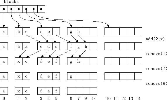
![]() arrays called blocks that are numbered
arrays called blocks that are numbered
![]() .
See Figure 2.5. Block
.
See Figure 2.5. Block ![]() contains
contains ![]() elements.
Therefore, all
elements.
Therefore, all
![]() blocks contain a total of
blocks contain a total of
  ArrayStack<T*> blocks;
  int n;
|
The elements of the list are laid out in the blocks as we might
expect. The list element with index 0 is stored in block 0, the
elements with list indices 1 and 2 are stored in block 1, the elements
with list indices 3, 4, and 5 are stored in block 2, and so on. The
main problem we have to address is that of determining, given an index
![]() , which block contains
, which block contains
![]() as well as the index corresponding to
as well as the index corresponding to
![]() within that block.
within that block.
Determining the index of
![]() within its block turns out to be easy. If
index
within its block turns out to be easy. If
index
![]() is in block
is in block
![]() , then the number of elements in blocks
, then the number of elements in blocks
![]() is
is
![]() . Therefore,
. Therefore,
![]() is stored at location
is stored at location
  int i2b(int i) {
      double db = (-3.0 + sqrt(9 + 8*i)) / 2.0;
      int b = (int)ceil(db);
      return b;
  }
With this out of the way, the
![]() and
and
![]() methods are straightforward. We first compute the appropriate block
methods are straightforward. We first compute the appropriate block
![]() and the appropriate index
and the appropriate index
![]() within the block and then perform the appropriate operation:
within the block and then perform the appropriate operation:
  T get(int i) {
      int b = i2b(i);
      int j = i - b*(b+1)/2;
      return blocks.get(b)[j];
  }
  T set(int i, T x) {
      int b = i2b(i);
      int j = i - b*(b+1)/2;
      T y = blocks.get(b)[j];
      blocks.get(b)[j] = x;
      return y;
  }
If we use any of the data structures in this chapter for representing the
![]() list, then
list, then
![]() and
and
![]() will each run in constant time.
will each run in constant time.
The
![]() method will, by now, look familiar. We first check if
our data structure is full, by checking if the number of blocks
method will, by now, look familiar. We first check if
our data structure is full, by checking if the number of blocks
![]() is such that
is such that
![]() and, if so, we call
and, if so, we call
![]() to add another block. With this done, we shift elements with indices
to add another block. With this done, we shift elements with indices
![]() to the right by one position to make room for the
new element with index
to the right by one position to make room for the
new element with index
![]() :
:
  void add(int i, T x) {
      int r = blocks.size();
      if (r*(r+1)/2 < n + 1) grow();
      n++;
      for (int j = n-1; j > i; j--)
              set(j, get(j-1));
      set(i, x);
  }
The
![]() method does what we expect. It adds a new block:
method does what we expect. It adds a new block:
  void grow() {
      blocks.add(blocks.size(), new T[blocks.size()+1]);
  }
Ignoring the cost of the
![]() operation, the cost of an
operation, the cost of an
![]() operation is dominated by the cost of shifting and is therefore
operation is dominated by the cost of shifting and is therefore
![]() , just like an
, just like an
![]() .
.
The
![]() operation is similar to
operation is similar to
![]() . It shifts the
elements with indices
. It shifts the
elements with indices
![]() left by one position and then,
if there is more than one empty block, it calls the
left by one position and then,
if there is more than one empty block, it calls the
![]() method
to remove all but one of the unused blocks:
method
to remove all but one of the unused blocks:
  T remove(int i) {
      T x = get(i);
      for (int j = i; j < n-1; j++)
              set(j, get(j+1));
      n--;
      int r = blocks.size();
      if ((r-2)*(r-1)/2 >= n) shrink();
      return x;
  }
  void shrink() {
      int r = blocks.size();
      while (r > 0 && (r-2)*(r-1)/2 >= n) {
              delete [] blocks.remove(blocks.size()-1);
              r--;
      }
  }
Once again, ignoring the cost of the
![]() operation, the cost of
a
operation, the cost of
a
![]() operation is dominated by the cost of shifting and is
therefore
operation is dominated by the cost of shifting and is
therefore
![]() .
.
The above analysis of
![]() and
and
![]() does not account for
the cost of
does not account for
the cost of
![]() and
and
![]() . Note that, unlike the
. Note that, unlike the
![]() operation,
operation,
![]() and
and
![]() do not do any
copying of data. They only allocate or free an array of size
do not do any
copying of data. They only allocate or free an array of size
![]() . In
some environments, this takes only constant time, while in others, it
may require
. In
some environments, this takes only constant time, while in others, it
may require
![]() time.
time.
We note that, immediately after a call to
![]() or
or
![]() , the
situation is clear. The final block is completely empty and all other
blocks are completely full. Another call to
, the
situation is clear. The final block is completely empty and all other
blocks are completely full. Another call to
![]() or
or
![]() will
not happen until at least
will
not happen until at least
![]() elements have been added or removed.
Therefore, even if
elements have been added or removed.
Therefore, even if
![]() and
and
![]() take
take
![]() time, this
cost can be amortized over at least
time, this
cost can be amortized over at least
![]()
![]() or
or
![]() operations, so that the amortized cost of
operations, so that the amortized cost of
![]() and
and
![]() is
is
![]() per operation.
per operation.
Next, we analyze the amount of extra space used by a
![]() .
In particular, we want to count any space used by a
.
In particular, we want to count any space used by a
![]() that is not an array element currently used to hold a list element. We call all such space wasted space.
that is not an array element currently used to hold a list element. We call all such space wasted space.
The
![]() operation ensures that a
operation ensures that a
![]() never has
more than 2 blocks that are not completely full. The number of blocks,
never has
more than 2 blocks that are not completely full. The number of blocks,
![]() , used by a
, used by a
![]() that stores
that stores
![]() elements therefore
satisfies
elements therefore
satisfies
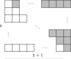
Next, we argue that this space usage is optimal for any data structure
that starts out empty and can support the addition of one item at a
time. More precisely, we will show that, at some point during the
addition of
![]() items, the data structure is wasting an amount of
space at least in
items, the data structure is wasting an amount of
space at least in
![]() (though it may be only wasted for a
moment).
(though it may be only wasted for a
moment).
Suppose we start with an empty data structure and we add
![]() items
one at a time. At the end of this process, all
items
one at a time. At the end of this process, all
![]() items are stored
in the structure and they are distributed among a collection of
items are stored
in the structure and they are distributed among a collection of
![]() memory blocks. If
memory blocks. If
![]() , then the data structure must be
using
, then the data structure must be
using
![]() pointers (or references) to keep track of these
pointers (or references) to keep track of these
![]() blocks,
and this is wasted space. On the other hand, if
blocks,
and this is wasted space. On the other hand, if
![]() then, by the pigeonhole principle, some block must have size at least
then, by the pigeonhole principle, some block must have size at least
![]() . Consider the moment at which this block was
first allocated. Immediately after it was allocated, this block was
empty, and was therefore wasting
. Consider the moment at which this block was
first allocated. Immediately after it was allocated, this block was
empty, and was therefore wasting
![]() space. Therefore, at some
point in time during the insertion of
space. Therefore, at some
point in time during the insertion of
![]() elements, the data structure was
wasting
elements, the data structure was
wasting
![]() space.
space.
The following theorem summarizes the performance of the
![]() data structure:
data structure:
The space (measured in words)3 used by a
![]() that stores
that stores
![]() elements is
elements is
![]() .
.
A reader who has had some exposure to models of computation may notice
that the
![]() , as described above, does not fit into
the usual word-RAM model of computation (Section 1.3) because it
requires taking square roots. The square root operation is generally
not considered a basic operation and is therefore not usually part of
the word-RAM model.
, as described above, does not fit into
the usual word-RAM model of computation (Section 1.3) because it
requires taking square roots. The square root operation is generally
not considered a basic operation and is therefore not usually part of
the word-RAM model.
In this section, we take time to show that the square root operation can
be implemented efficiently. In particular, we show that for any integer
![]() ,
,
![]() can be computed
in constant-time, after
can be computed
in constant-time, after
![]() preprocessing that creates two
arrays of length
preprocessing that creates two
arrays of length
![]() .
The following lemma shows that we can reduce the problem of computing the square root of
.
The following lemma shows that we can reduce the problem of computing the square root of
![]() to the square root of a related value
to the square root of a related value
![]() .
.
Start by restricting the problem a little, and assume that
![]() , so that
, so that
![]() , i.e.,
, i.e.,
![]() is an
integer having
is an
integer having
![]() bits in its binary representation. We can take
bits in its binary representation. We can take
![]() . Now,
. Now,
![]() satisfies
the conditions of Lemma 2.3, so
satisfies
the conditions of Lemma 2.3, so
![]() .
Furthermore,
.
Furthermore,
![]() has all of its lower-order
has all of its lower-order
![]() bits
equal to 0, so there are only
bits
equal to 0, so there are only
  int sqrt(int x, int r) {
    int s = sqrtab[x>>r/2];
    while ((s+1)*(s+1) <= x) s++; // executes at most twice
    return s;
  }
Now, this only works for
![]() and
and
![]() is a special table that only works for a particular value
of
is a special table that only works for a particular value
of
![]() . To overcome this, we could compute
. To overcome this, we could compute
![]() different
different
![]() arrays, one for each possible
value of
arrays, one for each possible
value of
![]() . The sizes of these tables form an exponential sequence whose largest value is at most
. The sizes of these tables form an exponential sequence whose largest value is at most
![]() , so the total size of all tables is
, so the total size of all tables is
![]() .
.
However, it turns out that more than one
![]() array is unnecessary;
we only need one
array is unnecessary;
we only need one
![]() array for the value
array for the value
![]() . Any value
. Any value
![]() with
with
![]() can be upgraded
by multiplying
can be upgraded
by multiplying
![]() by
by
![]() and using the equation
and using the equation
  int sqrt(int x) {
    int rp = log(x);
    int upgrade = ((r-rp)/2) * 2;
    int xp = x << upgrade;  // xp has r or r-1 bits
    int s = sqrtab[xp>>(r/2)] >> (upgrade/2);
    while ((s+1)*(s+1) <= x) s++;  // executes at most twice
    return s;
  }
Something we have taken for granted thus far is the question of how
to compute
![]() . Again, this is a problem that can be solved
with an array,
. Again, this is a problem that can be solved
with an array,
![]() , of size
, of size
![]() . In this case, the
code is particularly simple, since
. In this case, the
code is particularly simple, since
![]() is just the
index of the most significant 1 bit in the binary representation of
is just the
index of the most significant 1 bit in the binary representation of
![]() .
This means that, for
.
This means that, for
![]() , we can right-shift the bits of
, we can right-shift the bits of
![]() by
by
![]() positions before using it as an index into
positions before using it as an index into
![]() .
The following code does this using an array
.
The following code does this using an array
![]() of size
of size ![]() to compute
to compute
![]() for all
for all
![]() in the range
in the range
![]()
  int log(int x) {
    if (x >= halfint)
      return 16 + logtab[x>>16];
    return logtab[x];
  }
Finally, for completeness, we include the following code that initializes
![]() and
and
![]() :
:
  void inittabs() {
    sqrtab = new int[1<<(r/2)];
    logtab = new int[1<<(r/2)];
    for (int d = 0; d < r/2; d++)
      for (int k = 0; k < 1<<d; k++)
        logtab[1<<d+k] = d;
    int s = 1<<(r/4);                    // sqrt(2^(r/2))
    for (int i = 0; i < 1<<(r/2); i++) {
      if ((s+1)*(s+1) <= i << (r/2)) s++; // sqrt increases
      sqrtab[i] = s;
    }
  }
To summarize, the computations done by the
![]() method can be
implemented in constant time on the word-RAM using
method can be
implemented in constant time on the word-RAM using
![]() extra
memory to store the
extra
memory to store the
![]() and
and
![]() arrays. These arrays can be
rebuilt when
arrays. These arrays can be
rebuilt when
![]() increases or decreases by a factor of 2, and the cost
of this rebuilding can be amortized over the number of
increases or decreases by a factor of 2, and the cost
of this rebuilding can be amortized over the number of
![]() and
and
![]() operations that caused the change in
operations that caused the change in
![]() in the same way that
the cost of
in the same way that
the cost of
![]() is analyzed in the
is analyzed in the
![]() implementation.
implementation.