Next: 7.2 : A Randomized Up: 7. Random Binary Search Previous: 7. Random Binary Search Contents
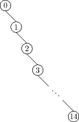
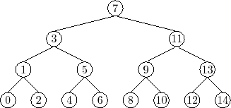
Consider the two binary search trees shown in Figure 7.1. The one
on the left is a list and the other is a perfectly balanced binary search
tree. The one on the left has height
![]() and the one on the right
has height three.
and the one on the right
has height three.
Imagine how these two trees could have been constructed. The one on
the left occurs if we start with an empty
![]() and add
the sequence
and add
the sequence
The above example gives some anecdotal evidence that, if we choose a
random permutation of
![]() , and add it into a binary search
tree then we are more likely to get a very balanced tree (the right
side of Figure 7.1) than we are to get a very unbalanced tree
(the left side of Figure 7.1).
, and add it into a binary search
tree then we are more likely to get a very balanced tree (the right
side of Figure 7.1) than we are to get a very unbalanced tree
(the left side of Figure 7.1).
We can formalize this notion by studying random binary search trees.
A random binary search tree of size
![]() is obtained in the
following way: Take a random permutation
is obtained in the
following way: Take a random permutation
![]() of
of
![]() and add its elements, one by one, into a
and add its elements, one by one, into a
![]() .
.
Note that the values
![]() could be replaced by any ordered
set of
could be replaced by any ordered
set of
![]() elements without changing any of the properties of the
random binary search tree. The element
elements without changing any of the properties of the
random binary search tree. The element
![]() is
simply standing in for the element of rank
is
simply standing in for the element of rank
![]() in an ordered set of
size
in an ordered set of
size
![]() .
.
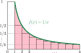
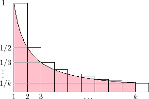
Before we can present our main result about random binary search trees,
we must take some time for a short digression to discuss a type of number
that comes up frequently when studying randomized structures. For a
non-negative integer, ![]() , the
, the ![]() -th harmonic number, denoted
-th harmonic number, denoted
![]() , is defined as
, is defined as
We will prove Lemma 7.1 in the next section. For now, consider what
the two parts of Lemma 7.1 tell us. The first part tells us that if
we search for an element in a tree of size
![]() , then the expected length
of the search path is at most
, then the expected length
of the search path is at most
![]() . The second part tells
us the same thing about searching for a value not stored in the tree.
When we compare the two parts of the lemma, we see that it is only
slightly faster to search for something that is in a tree compared to
something that is not in a tree.
. The second part tells
us the same thing about searching for a value not stored in the tree.
When we compare the two parts of the lemma, we see that it is only
slightly faster to search for something that is in a tree compared to
something that is not in a tree.
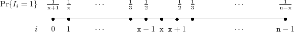
The key observation needed to prove Lemma 7.1 is the following: The
search path for a value
![]() in the open interval
in the open interval
![]() in a random binary search tree,
in a random binary search tree, ![]() , contains
the node with key
, contains
the node with key
![]() if and only if, in the random permutation
used to create
if and only if, in the random permutation
used to create ![]() ,
, ![]() appears before any of
appears before any of
![]() .
.
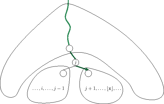
To see this, refer to Figure 7.3 and notice that, until
some value in
![]() is added, the search
paths for each value in the open interval
is added, the search
paths for each value in the open interval
![]() are identical. (Remember that for two search values to have
different search paths, there must be some element in the tree that
compares differently with them.) Let
are identical. (Remember that for two search values to have
different search paths, there must be some element in the tree that
compares differently with them.) Let ![]() be the first element in
be the first element in
![]() to appear in the random permutation.
Notice that
to appear in the random permutation.
Notice that ![]() is now and will always be on the search path for
is now and will always be on the search path for
![]() .
If
.
If ![]() then the node
then the node
![]() containing
containing ![]() is created before the
node
is created before the
node
![]() that contains
that contains ![]() . Later, when
. Later, when ![]() is added, it will be
added to the subtree rooted at
is added, it will be
added to the subtree rooted at
![]() , since
, since ![]() . On the other
hand, the search path for
. On the other
hand, the search path for
![]() will never visit this subtree because it
will proceed to
will never visit this subtree because it
will proceed to
![]() after visiting
after visiting
![]() .
.
|
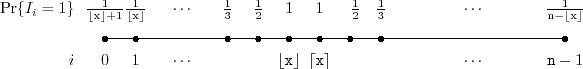
Similarly, for
![]() ,
, ![]() appears in the search path for
appears in the search path for
![]() if and only if
if and only if ![]() appears before any of
appears before any of
![]() in the random permutation used to
create
in the random permutation used to
create ![]() .
.
Notice that, if we start with a random permutation of
![]() ,
then the subsequences containing only
,
then the subsequences containing only
![]() and
and
![]() are also random
permutations of their respective elements. Each element, then, in the
subsets
are also random
permutations of their respective elements. Each element, then, in the
subsets
![]() and
and
![]() is equally likely to appear before
any other in its subset in the random permutation used to create
is equally likely to appear before
any other in its subset in the random permutation used to create ![]() .
So we have
.
So we have
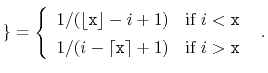
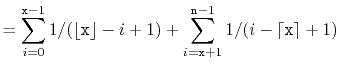
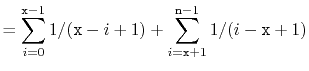
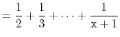
With this observation, the proof of Lemma 7.1 involves some simple calculations with harmonic numbers:
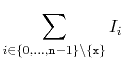
![$\displaystyle \mathrm{E}\left[\sum_{i=0}^{\ensuremath{\mathtt{x}}-1} I_i + \sum_{i=\ensuremath{\mathtt{x}}+1}^{\ensuremath{\mathtt{n}}-1} I_i\right]$](img1029.png) |
![$\displaystyle = \sum_{i=0}^{\ensuremath{\mathtt{x}}-1} \mathrm{E}\left[I_i\righ...
...nsuremath{\mathtt{x}}+1}^{\ensuremath{\mathtt{n}}-1} \mathrm{E}\left[I_i\right]$](img1030.png) |
|
 |
||
 |
||
 |
||
 |
||
|
The following theorem summarizes the performance of a random binary search tree: