Next: 2.4 ArrayDeque: Fast Deque Up: 2. Array-Based Lists Previous: 2.2 FastArrayStack: An Optimized Contents Index
In this section, we present the ArrayQueue data structure, which
implements a FIFO (first-in-first-out) queue; elements are removed (using
the
![]() operation) from the queue in the same order they are added
(using the
operation) from the queue in the same order they are added
(using the
![]() operation).
operation).
Notice that an ArrayStack is a poor choice for an implementation of a
FIFO queue. It is not a good choice because we must choose one end of
the list upon which to add elements and then remove elements from the
other end. One of the two operations must work on the head of the list,
which involves calling
![]() or
or
![]() with a value of
with a value of
![]() .
This gives a running time proportional to
.
This gives a running time proportional to
![]() .
.
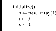
To obtain an efficient array-based implementation of a queue, we
first notice that the problem would be easy if we had an infinite
array
![]() . We could maintain one index
. We could maintain one index
![]() that keeps track of the
next element to remove and an integer
that keeps track of the
next element to remove and an integer
![]() that counts the number of
elements in the queue. The queue elements would always be stored in
that counts the number of
elements in the queue. The queue elements would always be stored in
Of course, the problem with this solution is that it requires an infinite
array. An ArrayQueue simulates this by using a finite array
![]() and modular arithmetic.
This is the kind of arithmetic used when
we are talking about the time of day. For example 10:00 plus five
hours gives 3:00. Formally, we say that
and modular arithmetic.
This is the kind of arithmetic used when
we are talking about the time of day. For example 10:00 plus five
hours gives 3:00. Formally, we say that
More generally, for an integer ![]() and positive integer
and positive integer ![]() ,
, ![]() is the unique integer
is the unique integer
![]() such that
such that
![]() for
some integer
for
some integer ![]() . Less formally, the value
. Less formally, the value ![]() is the remainder we get
when we divide
is the remainder we get
when we divide ![]() by
by ![]() .
In many programming languages, including C, C++, and Java,
the mod operate is represented using the % symbol.
.
In many programming languages, including C, C++, and Java,
the mod operate is represented using the % symbol.
Modular arithmetic is useful for simulating an infinite array,
since
![]() always gives a value in the range
always gives a value in the range
![]() . Using modular arithmetic we can store the
queue elements at array locations
. Using modular arithmetic we can store the
queue elements at array locations
The only remaining thing to worry about is taking care that the number
of elements in the ArrayQueue does not exceed the size of
![]() .
.
A sequence of
![]() and
and
![]() operations on an ArrayQueue is
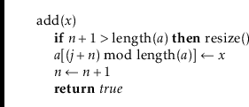
illustrated in Figure 2.2. To implement
operations on an ArrayQueue is
illustrated in Figure 2.2. To implement
![]() , we first
check if
, we first
check if
![]() is full and, if necessary, call
is full and, if necessary, call
![]() to increase
the size of
to increase
the size of
![]() . Next, we store
. Next, we store
![]() in
in
![]() and increment
and increment
![]() .
.
![\includegraphics[scale=0.90909]{figs-python/arrayqueue}](img689.png)
|
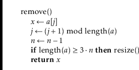
To implement
![]() , we first store
, we first store
![]() so that we can return
it later. Next, we decrement
so that we can return
it later. Next, we decrement
![]() and increment
and increment
![]() (modulo
(modulo
![]() )
by setting
)
by setting
![]() . Finally, we return the stored
value of
. Finally, we return the stored
value of
![]() . If necessary, we may call
. If necessary, we may call
![]() to decrease the
size of
to decrease the
size of
![]() .
.
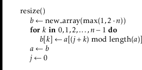
Finally, the
![]() operation is very similar to the
operation is very similar to the
![]() operation of ArrayStack. It allocates a new array,
operation of ArrayStack. It allocates a new array,
![]() , of size
, of size
![]() and copies
and copies
The following theorem summarizes the performance of the ArrayQueue data structure: