The running times of the depth-first-search and breadth-first-search
algorithms are somewhat overstated by the Theorems 12.3 and
12.4. Define
 as the number of vertices,
 ,
of
,
of  , for which there exists a path from
 to
to
 . Define
 as the number of edges that have these vertices as their sources.
Then the following theorem is a more precise statement of the running
times of the breadth-first-search and depth-first-search algorithms.
(This more refined statement of the running time is useful in some of
the applications of these algorithms outlined in the exercises.)
as the number of edges that have these vertices as their sources.
Then the following theorem is a more precise statement of the running
times of the breadth-first-search and depth-first-search algorithms.
(This more refined statement of the running time is useful in some of
the applications of these algorithms outlined in the exercises.)
Theorem 12..5
When given as input a Graph,
 , that is implemented using the
AdjacencyLists data structure, the
, that is implemented using the
AdjacencyLists data structure, the
 ,
,
 and
and
 algorithms each run in
 time.
time.
Breadth-first search seems to have been discovered independently by
Moore [52] and Lee [49] in the contexts of maze exploration
and circuit routing, respectively.
Adjacency-list representations of graphs were presented by
Hopcroft and Tarjan [40] as an alternative to the (then more
common) adjacency-matrix representation. This representation, as well as
depth-first-search, played a major part in the celebrated Hopcroft-Tarjan
planarity testing algorithm
that can determine, in
 time, if
a graph can be drawn, in the plane, and in such a way that no pair of
edges cross each other [41].
time, if
a graph can be drawn, in the plane, and in such a way that no pair of
edges cross each other [41].
In the following exercises, an undirected graph is one in which, for
every
 and
and
 , the edge
 is present if and only if the
edge
is present if and only if the
edge
 is present.
Exercise 12..1
Draw an adjacency list representation and an adjacency matrix
representation of the graph in Figure
12.7.
Figure 12.7:
An example graph.
|
![\includegraphics[scale=0.90909]{figs-python/graph-example2}](img4821.png) |
Exercise 12..2
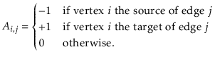
The
incidence matrix representation of a graph,

, is an

matrix,

, where
- Draw the incident matrix representation of the graph in
Figure 12.7.
- Design, analyze and implement an incidence matrix representation
of a graph. Be sure to analyze the space, the cost of
 ,
,
 ,
,
 ,
,
 ,
and
,
and
 .
.
Exercise 12..3
Illustrate an execution of the

and

on the graph,

,
in Figure
12.7.
Exercise 12..4
Let

be an undirected graph. We say

is
connected if,
for every pair of vertices

and

in

, there is a path from

to

(since

is undirected, there is also a path from

to

). Show how to test if

is connected in

time.
Exercise 12..5
Let

be an undirected graph. A
connected-component labelling
of

partitions the vertices of

into maximal sets, each of which
forms a connected subgraph. Show how to compute a connected component
labelling of

in

time.
Exercise 12..6
Let

be an undirected graph. A
spanning forest of

is a
collection of trees, one per component, whose edges are edges of

and whose vertices contain all vertices of

. Show how to compute
a spanning forest of of

in

time.
Exercise 12..7
We say that a graph

is
strongly-connected if, for every
pair of vertices

and

in

, there is a path from

to

. Show how to test if

is strongly-connected in

time.
Exercise 12..8
Given a graph

and some special vertex

, show how
to compute the length of the shortest path from

to

for every
vertex

.
Exercise 12..9
Give a (simple) example where the

code visits the nodes of a
graph in an order that is different from that of the

code.
Write a version of

that always visits nodes in exactly
the same order as

. (Hint: Just start tracing the execution
of each algorithm on some graph where

is the source of more than
1 edge.)
Exercise 12..10
A
universal sink in a graph

is a vertex that is the target
of

edges and the source of no edges.
12.1 Design and implement an algorithm that tests if a graph

, represented
as an AdjacencyMatrix, has a universal sink. Your algorithm should
run in

time.
Footnotes
- ... edges.12.1
- A universal sink,
 , is also sometimes called a celebrity: Everyone in the room
recognizes
, is also sometimes called a celebrity: Everyone in the room
recognizes
 , but
, but
 doesn't recognize anyone else in the room.
opendatastructures.org