Next: 12.2 AdjacencyLists: A Graph Up: 12. Graphs Previous: 12. Graphs Contents Index
An adjacency matrix is a way of representing an
![]() vertex graph
vertex graph
![]() by an
by an
![]() matrix,
matrix,
![]() , whose entries are boolean
values.
, whose entries are boolean
values.
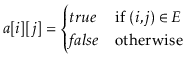
The matrix entry
![]() is defined as
is defined as
In this representation, the operations
![]() ,
,
![]() , and
, and
![]() just
involve setting or reading the matrix entry
just
involve setting or reading the matrix entry
![]() :
:
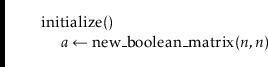
![\begin{leftbar}
\begin{flushleft}
\hspace*{1em} \ensuremath{\mathrm{add\_edge}(\...
...it{a}}[\ensuremath{\mathit{i}}]}[\ensuremath{j}]\\
\end{flushleft}\end{leftbar}](img4572.png)
These operations clearly take constant time per operation.
![\includegraphics[scale=0.90909]{figs-python/graph}](img4573.png)
|
Where the adjacency matrix performs poorly is with the
![]() and
and
![]() operations. To implement these, we must scan all
operations. To implement these, we must scan all
![]() entries in the corresponding row or column of
entries in the corresponding row or column of
![]() and gather up all the
indices,
and gather up all the
indices,
![]() , where
, where
![]() , respectively
, respectively
![]() , is true.
These operations clearly take
, is true.
These operations clearly take
![]() time per operation.
time per operation.
Another drawback of the adjacency matrix representation is that it
is large. It stores an
![]() boolean matrix, so it requires at
least
boolean matrix, so it requires at
least
![]() bits of memory. The implementation here uses a matrix
of values so it actually uses on the
order of
bits of memory. The implementation here uses a matrix
of values so it actually uses on the
order of
![]() bytes of memory. A more careful implementation, which
packs
bytes of memory. A more careful implementation, which
packs
![]() boolean values into each word of memory, could reduce this
space usage to
boolean values into each word of memory, could reduce this
space usage to
![]() words of memory.
words of memory.
Despite its high memory requirements and poor performance of the
![]() and
and
![]() operations, an AdjacencyMatrix can still be useful for
some applications. In particular, when the graph
operations, an AdjacencyMatrix can still be useful for
some applications. In particular, when the graph ![]() is dense,
i.e., it has close to
is dense,
i.e., it has close to
![]() edges, then a memory usage of
edges, then a memory usage of
![]() may be acceptable.
may be acceptable.
The AdjacencyMatrix data structure is also commonly used because
algebraic operations on the matrix
![]() can be used to efficiently compute
properties of the graph
can be used to efficiently compute
properties of the graph ![]() . This is a topic for a course on algorithms,
but we point out one such property here: If we treat the entries of
. This is a topic for a course on algorithms,
but we point out one such property here: If we treat the entries of
![]() as integers (1 for
as integers (1 for
![]() and 0 for
and 0 for
![]() ) and multiply
) and multiply
![]() by itself
using matrix multiplication then we get the matrix
by itself
using matrix multiplication then we get the matrix
![]() . Recall,
from the definition of matrix multiplication, that
. Recall,
from the definition of matrix multiplication, that
![$\displaystyle \ensuremath{\ensuremath{\ensuremath{\mathit{a}}\ensuremath{\oplus...
...{\ensuremath{\mathit{a}}[\ensuremath{\mathit{k}}]}[\ensuremath{j}]} \enspace .
$](img4606.png)
opendatastructures.org