Next: 5.2 : Linear Probing Up: 5. Hash Tables Previous: 5. Hash Tables Contents Index
A
![]() data structure uses hashing with chaining to store
data as an array,
data structure uses hashing with chaining to store
data as an array,
![]() , of lists. An integer,
, of lists. An integer,
![]() , keeps track of the
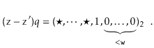
total number of items in all lists (see Figure 5.1):
, keeps track of the
total number of items in all lists (see Figure 5.1):
array<List> t; int n;The hash value of a data item
To add an element,
![]() , to the hash table, we first check if
the length of
, to the hash table, we first check if
the length of
![]() needs to be increased and, if so, we grow
needs to be increased and, if so, we grow
![]() .
With this out of the way we hash
.
With this out of the way we hash
![]() to get an integer,
to get an integer,
![]() , in the
range
, in the
range
![]() , and we append
, and we append
![]() to the list
to the list
![]() :
:
  bool add(T x) {
    if (find(x) != null) return false;
    if (n+1 > t.length) resize();
    t[hash(x)].add(x);
    n++;
    return true;
  }
Growing the table,
if necessary, involves doubling the length of
![[*]](crossref.png) ).
).
Besides growing, the only other work done when adding a new value
![]() to a
to a
![]() involves appending
involves appending
![]() to the list
to the list
![]() . For
any of the list implementations described in Chapters 2
or 3, this takes only constant time.
. For
any of the list implementations described in Chapters 2
or 3, this takes only constant time.
To remove an element,
![]() , from the hash table, we iterate over the list
, from the hash table, we iterate over the list
![]() until we find
until we find
![]() so that we can remove it:
so that we can remove it:
  T remove(T x) {
    int j = hash(x);
    for (int i = 0; i < t[j].size(); i++) {
      T y = t[j].get(i);
      if (x == y) {
        t[j].remove(i);
        n--;
        return y;
      }
    }
    return null;
  }
This takes
Searching for the element
![]() in a hash table is similar. We perform
a linear search on the list
in a hash table is similar. We perform
a linear search on the list
![]() :
:
  T find(T x) {
    int j = hash(x);
    for (int i = 0; i < t[j].size(); i++)
      if (x == t[j].get(i))
        return t[j].get(i);
    return null;
  }
Again, this takes time proportional to the length of the list
The performance of a hash table depends critically on the choice of the
hash function. A good hash function will spread the elements evenly
among the
![]() lists, so that the expected size of the list
lists, so that the expected size of the list
![]() is
is
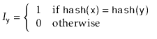
![]() . On the other hand, a bad
hash function will hash all values (including
. On the other hand, a bad
hash function will hash all values (including
![]() ) to the same table
location, in which case the size of the list
) to the same table
location, in which case the size of the list
![]() will be
will be
![]() .
In the next section we describe a good hash function.
.
In the next section we describe a good hash function.
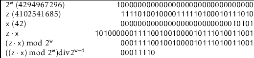
Multiplicative hashing is an efficient method of generating hash
values based on modular arithmetic (discussed in Section 2.3)
and integer division. It uses the ![]() operator, which calculates
the integral part of a quotient, while discarding the remainder.
Formally, for any integers
operator, which calculates
the integral part of a quotient, while discarding the remainder.
Formally, for any integers ![]() and
and ![]() ,
,
![]() .
.
In multiplicative hashing, we use a hash table of size
![]() for some
integer
for some
integer
![]() (called the dimension). The formula for hashing an
integer
(called the dimension). The formula for hashing an
integer
![]() is
is
  int hash(T x) {
    return ((unsigned)(z * hashCode(x))) >> (w-d);
  }
The following lemma, whose proof is deferred until later in this section, shows that multiplicative hashing does a good job of avoiding collisions:
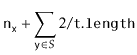
With Lemma 5.1, the performance of
![]() , and
, and
![]() are easy to analyze:
are easy to analyze:
![$\displaystyle \mathrm{E}\left[\ensuremath{\mathtt{n}}_{\ensuremath{\mathtt{x}}} + \sum_{\ensuremath{\mathtt{y}}\in S} I_{\ensuremath{\mathtt{y}}}\right]$](img2498.png) |
|||
![$\displaystyle \ensuremath{\mathtt{n}}_{\ensuremath{\mathtt{x}}} + \sum_{\ensuremath{\mathtt{y}}\in S} \mathrm{E}[I_{\ensuremath{\mathtt{y}}} ]$](img2500.png) |
|||
 |
|||
 |
|||
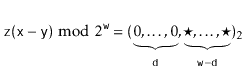
Now, we want to prove Lemma 5.1, but first we need a
result from number theory. In the following proof, we use the notation
![]() to denote
to denote
![]() , where each
, where each ![]() is a bit, either 0 or 1. In other words,
is a bit, either 0 or 1. In other words,
![]() is
the integer whose binary representation is given by
is
the integer whose binary representation is given by
![]() .
We use
.
We use ![]() to denote a bit of unknown value.
to denote a bit of unknown value.
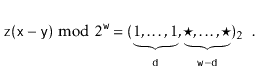
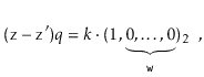
Suppose, for the sake of contradiction, that there are two such values
![]() and
and
![]() , with
, with
![]() . Then
. Then
Furthermore ![]() , since
, since ![]() and
and
![]() . Since
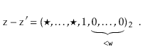
. Since ![]() is odd, it has no trailing 0's in its binary representation:
is odd, it has no trailing 0's in its binary representation:
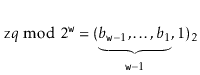
The utility of Lemma 5.3 comes from the following
observation: If
![]() is chosen uniformly at random from
is chosen uniformly at random from ![]() , then
, then
![]() is uniformly distributed over
is uniformly distributed over ![]() . In the following proof, it helps
to think of the binary representation of
. In the following proof, it helps
to think of the binary representation of
![]() , which consists of
, which consists of
![]() random bits followed by a 1.
random bits followed by a 1.
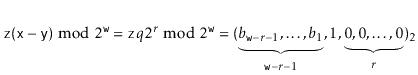
Let ![]() be the unique odd integer such that
be the unique odd integer such that
![]() for some integer
for some integer ![]() . By
Lemma 5.3, the binary representation of
. By
Lemma 5.3, the binary representation of
![]() has
has
![]() random bits, followed by a 1:
random bits, followed by a 1:
The following theorem summarizes the performance of a
![]() data structure:
data structure:
Furthermore, beginning with an empty
![]() , any sequence of
, any sequence of
![]()
![]() and
and
![]() operations results in a total of
operations results in a total of ![]() time spent during all calls to
time spent during all calls to
![]() .
.
![\includegraphics[width=\textwidth ]{figs/chainedhashtable}](img2413.png)