12.2 AdjacencyLists: A Graph as a Collection of Lists

Adjacency list representations of graphs take a more vertex-centric approach. There are many possible implementations of adjacency lists. In this section, we present a simple one. At the end of the section, we discuss different possibilities. In an adjacency list representation, the graph $G=(V,E)$ is represented as an array, $\ensuremath{\ensuremath{\mathit{adj}}}$, of lists. The list $\ensuremath{\ensuremath{\mathit{adj}}[\ensuremath{\mathit{i}}]}$ contains a list of all the vertices adjacent to vertex $\ensuremath{\ensuremath{\mathit{i}}}$. That is, it contains every index $\ensuremath{\ensuremath{\mathit{j}}}$ such that $\ensuremath{\ensuremath{(\ensuremath{\mathit{i}},\ensuremath{\mathit{j}})}}\in E$.

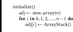
(An example is shown in Figure 12.3.) In this particular implementation, we represent each list in $\ensuremath{\ensuremath{\mathit{adj}}}$ as ArrayStack, because we would like constant time access by position. Other options are also possible. Specifically, we could have implemented $\ensuremath{\ensuremath{\mathit{adj}}}$ as a DLList.

Figure 12.3: A graph and its adjacency lists

0	1	2	3	4	5	6	7	8	9	10	11
1	0	1	2	0	1	5	6	4	8	9	10
4	2	3	7	5	2	2	3	9	5	6	7
	6	6		8	6	7	11		10	11
	5				9	10
					4

The $\ensuremath{\mathrm{add\_edge}(\ensuremath{\mathit{i}},\ensuremath{\mathit{j}})}$ operation just appends the value $\ensuremath{\ensuremath{\mathit{j}}}$ to the list $\ensuremath{\ensuremath{\mathit{adj}}[\ensuremath{\mathit{i}}]}$:

This takes constant time.

The $\ensuremath{\mathrm{remove\_edge}(\ensuremath{\mathit{i}},\ensuremath{\mathit{j}})}$ operation searches through the list $\ensuremath{\ensuremath{\mathit{adj}}[\ensuremath{\mathit{i}}]}$ until it finds $\ensuremath{\ensuremath{\mathit{j}}}$ and then removes it:

This takes $O(\deg(\ensuremath{\ensuremath{\ensuremath{\mathit{i}}}}))$ time, where $\deg(\ensuremath{\ensuremath{\ensuremath{\mathit{i}}}})$ (the degree of $\ensuremath{\ensuremath{\ensuremath{\mathit{i}}}}$) counts the number of edges in $E$ that have $\ensuremath{\ensuremath{\ensuremath{\mathit{i}}}}$ as their source.

The $\ensuremath{\mathrm{has\_edge}(\ensuremath{\mathit{i}},\ensuremath{\mathit{j}})}$ operation is similar; it searches through the list $\ensuremath{\ensuremath{\mathit{adj}}[\ensuremath{\mathit{i}}]}$ until it finds $\ensuremath{\ensuremath{\mathit{j}}}$ (and returns true), or reaches the end of the list (and returns false):

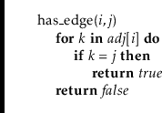
This also takes $O(\deg(\ensuremath{\ensuremath{\ensuremath{\mathit{i}}}}))$ time.

The $\ensuremath{\mathrm{out\_edges}(\ensuremath{\mathit{i}})}$ operation is very simple; it returns the list $\ensuremath{\ensuremath{\mathit{adj}}[\ensuremath{\mathit{i}}]}$ :

The $\ensuremath{\mathrm{in\_edges}(\ensuremath{\mathit{i}})}$ operation is much more work. It scans over every vertex $j$ checking if the edge $\ensuremath{(\ensuremath{\mathit{i}},\ensuremath{\mathit{j}})}$ exists and, if so, adding $\ensuremath{\ensuremath{\mathit{j}}}$ to the output list:

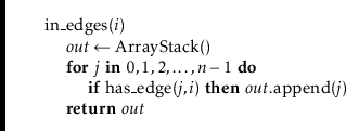
This operation is very slow. It scans the adjacency list of every vertex, so it takes $O(\ensuremath{\ensuremath{\ensuremath{\mathit{n}}}} + \ensuremath{\ensuremath{\ensuremath{\mathit{m}}}})$ time.

The following theorem summarizes the performance of the above data structure:

Theorem 12..2   The AdjacencyLists data structure implements the Graph interface. An AdjacencyLists supports the operations

• $\ensuremath{\mathrm{add\_edge}(\ensuremath{\mathit{i}},\ensuremath{\mathit{j}})}$ in constant time per operation;
• $\ensuremath{\mathrm{remove\_edge}(\ensuremath{\mathit{i}},\ensuremath{\mathit{j}})}$ and $\ensuremath{\mathrm{has\_edge}(\ensuremath{\mathit{i}},\ensuremath{\mathit{j}})}$ in $O(\deg(\ensuremath{\ensuremath{\ensuremath{\mathit{i}}}}))$ time per operation;
• $\ensuremath{\mathrm{in\_edges}(\ensuremath{\mathit{i}})}$ in $O(\ensuremath{\ensuremath{\ensuremath{\mathit{n}}}}+\ensuremath{\ensuremath{\ensuremath{\mathit{m}}}})$ time per operation.

The space used by a AdjacencyLists is $O(\ensuremath{\ensuremath{\ensuremath{\mathit{n}}}}+\ensuremath{\ensuremath{\ensuremath{\mathit{m}}}})$.

As alluded to earlier, there are many different choices to be made when implementing a graph as an adjacency list. Some questions that come up include:

• What type of collection should be used to store each element of $\ensuremath{\ensuremath{\mathit{adj}}}$? One could use an array-based list, a linked-list, or even a hashtable.
• Should there be a second adjacency list, $\ensuremath{\ensuremath{\mathit{inadj}}}$, that stores, for each $\ensuremath{\ensuremath{\mathit{i}}}$, the list of vertices, $\ensuremath{\ensuremath{\mathit{j}}}$, such that $\ensuremath{\ensuremath{(\ensuremath{\mathit{j}},\ensuremath{\mathit{i}})}}\in E$? This can greatly reduce the running-time of the $\ensuremath{\mathrm{in\_edges}(\ensuremath{\mathit{i}})}$ operation, but requires slightly more work when adding or removing edges.
• Should the entry for the edge $\ensuremath{(\ensuremath{\mathit{i}},\ensuremath{\mathit{j}})}$ in $\ensuremath{\ensuremath{\mathit{adj}}[\ensuremath{\mathit{i}}]}$ be linked by a reference to the corresponding entry in $\ensuremath{\ensuremath{\mathit{inadj}}[\ensuremath{\mathit{j}}]}$?
• Should edges be first-class objects with their own associated data? In this way, $\ensuremath{\ensuremath{\mathit{adj}}}$ would contain lists of edges rather than lists of vertices (integers).

Most of these questions come down to a tradeoff between complexity (and space) of implementation and performance features of the implementation.