Next: 12.2 AdjacencyLists: A Graph Up: 12. Graphs Previous: 12. Graphs Contents
An adjacency matrix is a way of representing an
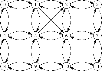
![]() vertex graph
vertex graph
![]() by an
by an
![]() matrix,
matrix,
![]() , whose entries are boolean
values.
, whose entries are boolean
values.
    int n;
    boolean[][] a;
    AdjacencyMatrix(int n0) {
        n = n0;
        a = new boolean[n][n];
    }
The matrix entry
![]() is defined as
is defined as
![$\displaystyle \ensuremath{\mathtt{a[i][j]}}=
\begin{cases}
\ensuremath{\math...
...(i,j)}}\in E$} \\
\ensuremath{\mathtt{false}} & \text{otherwise}
\end{cases}$](img1529.png)
With this representation, the
![]() ,
,
![]() , and
, and
![]() operations just
involve setting or reading the matrix entry
operations just
involve setting or reading the matrix entry
![]() :
:
    void addEdge(int i, int j) {
        a[i][j] = true;
    }
    void removeEdge(int i, int j) {
        a[i][j] = false;
    }
    boolean hasEdge(int i, int j) {
        return a[i][j];
    }
These operations clearly take constant time per operation.
|
Where the adjacency matrix performs poorly is with the
![]() and
and
![]() operations. To implement these, we must scan all
operations. To implement these, we must scan all
![]() entries in the corresponding row or column of
entries in the corresponding row or column of
![]() and gather up all the
indices,
and gather up all the
indices,
![]() , where
, where
![]() , respectively
, respectively
![]() , is true.
, is true.
    List<Integer> outEdges(int i) {
        List<Integer> edges = new ArrayList<Integer>();
        for (int j = 0; j < n; j++)
            if (a[i][j]) edges.add(j);
        return edges;
    }
    List<Integer> inEdges(int i) {
        List<Integer> edges = new ArrayList<Integer>();
        for (int j = 0; j < n; j++)
            if (a[j][i]) edges.add(j);
        return edges;
    }
These operations clearly take
Another drawback of the adjacency matrix representation is that it
is big. It stores an
![]() boolean matrix, so it requires at
least
boolean matrix, so it requires at
least
![]() bits of memory. The implementation here uses a matrix
of
bits of memory. The implementation here uses a matrix
of
![]() values so it actually uses on the
order of
values so it actually uses on the
order of
![]() bytes of memory. A more careful implementation, that
packs
bytes of memory. A more careful implementation, that
packs
![]() boolean values into each word of memory could reduce this
space usage to
boolean values into each word of memory could reduce this
space usage to
![]() words of memory.
words of memory.
Despite the high memory usage and poor performance of the
![]() and
and
![]() operations, an AdjacencyMatrix can still be useful for
some applications. In particular, when the graph
operations, an AdjacencyMatrix can still be useful for
some applications. In particular, when the graph ![]() is dense,
i.e., it has close to
is dense,
i.e., it has close to
![]() edges, then a memory usage of
edges, then a memory usage of
![]() may be acceptable.
may be acceptable.
The AdjacencyMatrix data structure is also commonly used because
algebraic operations on the matrix
![]() can be used to efficiently compute
properties of the graph
can be used to efficiently compute
properties of the graph ![]() . This is a topic for a course on algorithms,
but we point out one such property here: If we treat the entries of
. This is a topic for a course on algorithms,
but we point out one such property here: If we treat the entries of
![]() as integers (1 for
as integers (1 for
![]() and 0 for
and 0 for
![]() ) and multiply
) and multiply
![]() by itself
using matrix multiplication then we get the matrix
by itself
using matrix multiplication then we get the matrix
![]() . Recall,
from the definition of matrix multiplication, that
. Recall,
from the definition of matrix multiplication, that
![$\displaystyle \ensuremath{\mathtt{a^2[i][j]}} = \sum_{k=0}^{\ensuremath{\mathtt...
...1} \ensuremath{\mathtt{a[i][k]}}\cdot \ensuremath{\mathtt{a[k][j]}} \enspace .
$](img1535.png)
opendatastructures.org