Next: 13.3 : A Doubly-Logarithmic Up: 13. Data Structures for Previous: 13.1 : A digital Contents
The performance of the
![]() structure is not that impressive.
The number of elements,
structure is not that impressive.
The number of elements,
![]() , stored in the structure is at most
, stored in the structure is at most
![]() ,
so
,
so
![]() . In other words, any of the comparison-based
. In other words, any of the comparison-based
![]() structures described in other parts of this book are at least as efficient
as a
structures described in other parts of this book are at least as efficient
as a
![]() , and don't have the restriction of only being able to
store integers.
, and don't have the restriction of only being able to
store integers.
Next we describe the
![]() , which is just a
, which is just a
![]() with
with
![]() hash tables--one for each level of the trie. These hash tables
are used to speed up the
hash tables--one for each level of the trie. These hash tables
are used to speed up the
![]() operation to
operation to
![]() time.
Recall that the
time.
Recall that the
![]() operation in a
operation in a
![]() is almost complete
once we reach a node,
is almost complete
once we reach a node,
![]() , where the search path for
, where the search path for
![]() would like to
proceed to
would like to
proceed to
![]() (or
(or
![]() ) but
) but
![]() has no right (respectively,
left) child. At this point, the search uses
has no right (respectively,
left) child. At this point, the search uses
![]() to jump to a leaf,
to jump to a leaf,
![]() , of the
, of the
![]() and either return
and either return
![]() or its successor in the
linked list of leaves. An
or its successor in the
linked list of leaves. An
![]() speeds up the search process by
using binary search on the levels of the trie to locate the node
speeds up the search process by
using binary search on the levels of the trie to locate the node
![]() .
.
To use binary search, we need a way to determine if the node
![]() we are
looking for is above a particular level,
we are
looking for is above a particular level,
![]() , of if
, of if
![]() is at or below
level
is at or below
level
![]() . This information is given by the highest-order
. This information is given by the highest-order
![]() bits
in the binary representation of
bits
in the binary representation of
![]() ; these bits determine the search
path that
; these bits determine the search
path that
![]() takes from the root to level
takes from the root to level
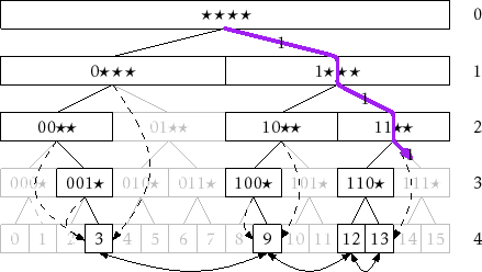
![]() . For an example,
refer to Figure 13.6; in this figure the last node,
. For an example,
refer to Figure 13.6; in this figure the last node,
![]() , on
search path for 14 (whose binary representation is 1110) is the node
labelled
, on
search path for 14 (whose binary representation is 1110) is the node
labelled
![]() at level 2 because there is no node labelled
at level 2 because there is no node labelled
![]() at level 3. Thus, we can label each node at level
at level 3. Thus, we can label each node at level
![]() with an
with an
![]() -bit integer. Then the node
-bit integer. Then the node
![]() we are searching for is at
or below level
we are searching for is at
or below level
![]() if and only if there is a node at level
if and only if there is a node at level
![]() whose
label matches the highest-order
whose
label matches the highest-order
![]() bits of
bits of
![]() .
.
|
In an
![]() , we store, for each
, we store, for each
![]() , all
the nodes at level
, all
the nodes at level
![]() in a
in a
![]() ,
,
![]() , that is implemented as a
hash table (Chapter 5). Using this
, that is implemented as a
hash table (Chapter 5). Using this
![]() allows us to check
in constant expected time if there is a node at level
allows us to check
in constant expected time if there is a node at level
![]() whose label
matches the highest-order
whose label
matches the highest-order
![]() bits of
bits of
![]() . In fact, we can even find
this node using
. In fact, we can even find
this node using
![]() .
.
The hash tables
![]() allow us to use binary search
to find
allow us to use binary search
to find
![]() . Initially, we know that
. Initially, we know that
![]() is at some level
is at some level
![]() with
with
![]() . We therefore initialize
. We therefore initialize
![]() and
and
![]() and repeatedly look at the hash table
and repeatedly look at the hash table
![]() , where
, where
![]() . If
. If
![]() contains a node whose label matches
contains a node whose label matches
![]() 's highest-order
's highest-order
![]() bits then we set
bits then we set
![]() (
(
![]() is at or below level
is at or below level
![]() ), otherwise we set
), otherwise we set
![]() (
(
![]() is above level
is above level
![]() ). This process
terminates when
). This process
terminates when
![]() , in which case we determine that
, in which case we determine that
![]() is
at level
is
at level
![]() . We then complete the
. We then complete the
![]() operation using
operation using
![]() and the doubly-linked list of leaves.
and the doubly-linked list of leaves.
  T find(T x) {
    int l = 0, h = w+1;
    unsigned ix = intValue(x);
    Node *v, *u = &r;
    while (h-l > 1) {
      int i = (l+h)/2;
      XPair<Node> p(ix >> (w-i));
      if ((v = t[i].find(p).u) == NULL) {
        h = i;
      } else {
        u = v;
        l = i;
      }
    }
    if (l == w) return u->x;
    Node *pred = (((ix >> (w-l-1)) & 1) == 1) ? u->jump : u->jump->prev;
    return (pred->next == &dummy) ? NULL : pred->next->x;
  }
Each iteration of the
The
![]() and
and
![]() methods for an
methods for an
![]() are almost
identical to the same methods in a
are almost
identical to the same methods in a
![]() . The only modifications
are for managing the hash tables
. The only modifications
are for managing the hash tables
![]() ,...,
,...,
![]() . During the
. During the
![]() operation, when a new node is created at level
operation, when a new node is created at level
![]() , this node
is added to
, this node
is added to
![]() . During a
. During a
![]() operation, when a node is
removed form level
operation, when a node is
removed form level
![]() , this node is removed from
, this node is removed from
![]() . Since adding
and removing from a hash table take constant expected time, this does
not increase the running times of
. Since adding
and removing from a hash table take constant expected time, this does
not increase the running times of
![]() and
and
![]() by more than
a constant factor. We omit a code listing or
by more than
a constant factor. We omit a code listing or
![]() and
and
![]() since
it is almost identical to the (long) code listing already provided
for the same methods in a
since
it is almost identical to the (long) code listing already provided
for the same methods in a
![]() .
.
The following theorem summarizes the performance of an
![]() :
:
opendatastructures.org